3.1 Optimization Algorithms

Motivation: MLE

Consider the simple linear regression model

$Y_i = \beta_0 + \beta X_i +\varepsilon_i,\quad \varepsilon_i\overset{iid}{\sim}N(0,\sigma^2)$

It follows that $Y_i\overset{ind}{\sim}N(\beta_0+\beta X_i,\sigma^2)$ , and each $Y_i$ has pdf:

$f(Y_i|X_i,\beta_0, \beta,\sigma^2)=\frac{1}{\sqrt{2\pi\sigma^2}}\exp\left( -\frac{(Y_i-\beta_0-\beta X_i)^2}{2\sigma^2}\right)$

For observed values $(y_1,x_1),(y_2,x_2)...,(y_n,x_n)$ , assuming independence of $y_i$ s, the likelihood function is given by:

$L(\beta_0, \beta, \sigma^2)=\prod_{i=1}^n\frac{1}{\sqrt{2\pi\sigma^2}}\exp\left( -\frac{(y_i-\beta_0-\beta x_i)^2}{2\sigma^2}\right)$

When obtaining the values of $\beta_0,\beta,\sigma^2$ that maximizes this likelihood function, we are lucky that this has a closed form solution, which are:

$\hat{\beta}_0 = \bar{y}-\hat{\beta}\bar{x}\\ \hat{\beta} = \frac{\sum (x_i-\bar{x})(y_i-\bar{y})}{\sum(x_i-\bar{x})}$

In this example, the maximization of the likelihood was simple because the solution was available in closed form.

However, in most other cases, there will not be a closed form solution and some specific algorithm will be needed to maximize the likelihood.

A likelihood function that has no closed form solution for the maximum?

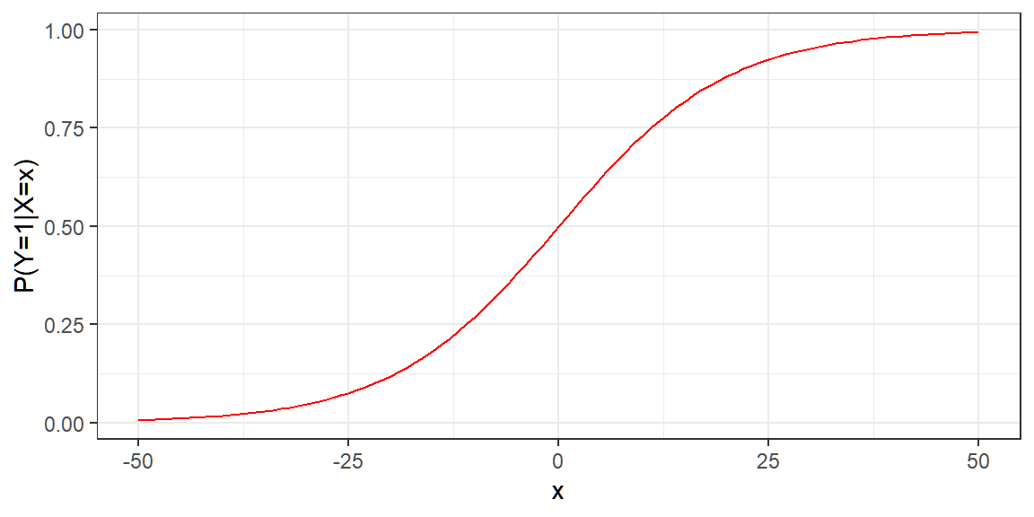
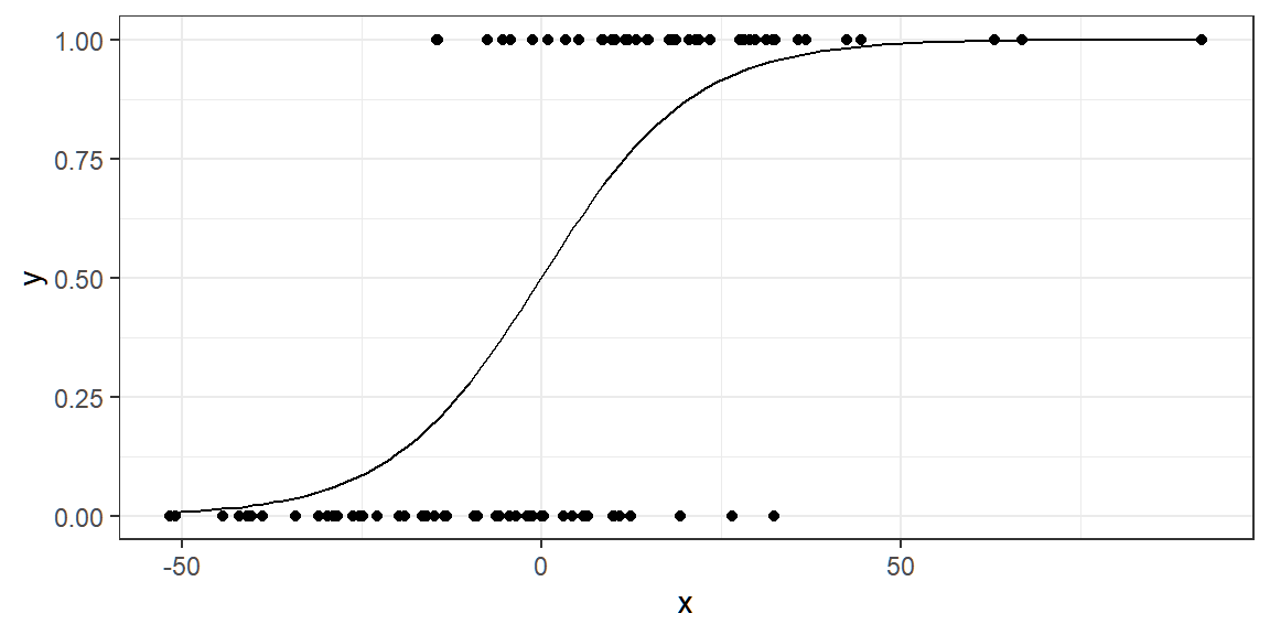
Let $Y$ be a binary response, and let $\pi(x)=P(Y=1|X=x)=1-P(Y=0|X=x)$ . A model for the probability of success of $Y$ is given by the logistic regression model:

$\pi(x) = \frac{\exp(\beta x)}{1+\exp (\beta x)}$

If $\beta=0.1$ , then the probability of success of $y$ based on different values of $x$ can be graphed as follows:

Suppose we have the following dataset generated from the above model:

ABCDEFGHIJ0123456789

y <dbl>	x <dbl>
1	31.3680213
1	42.6021356
1	22.0080756
1	-14.5386236
1	-4.2297142
0	26.6194716
1	17.9593872
1	0.9560583
0	-26.2415985
1	5.3078376

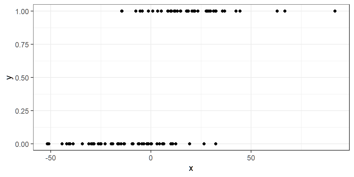
We are interested in estimating $\beta$ using maximum likelihood estimation.

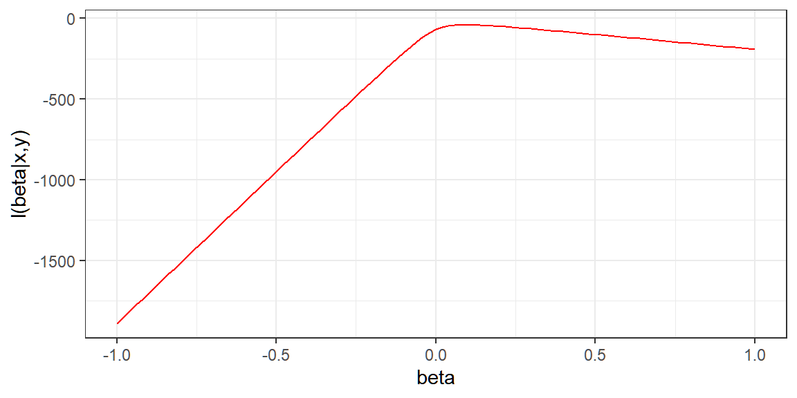
The final form of the log-likelihood function which is to be optimized can be derived as

$\ell(\beta|x_i,y_i)=\sum_{i=1}^n [y_i\beta x_i-\log(1+e^{\beta x_i})]$

See Agresti (2013) for full derivation.

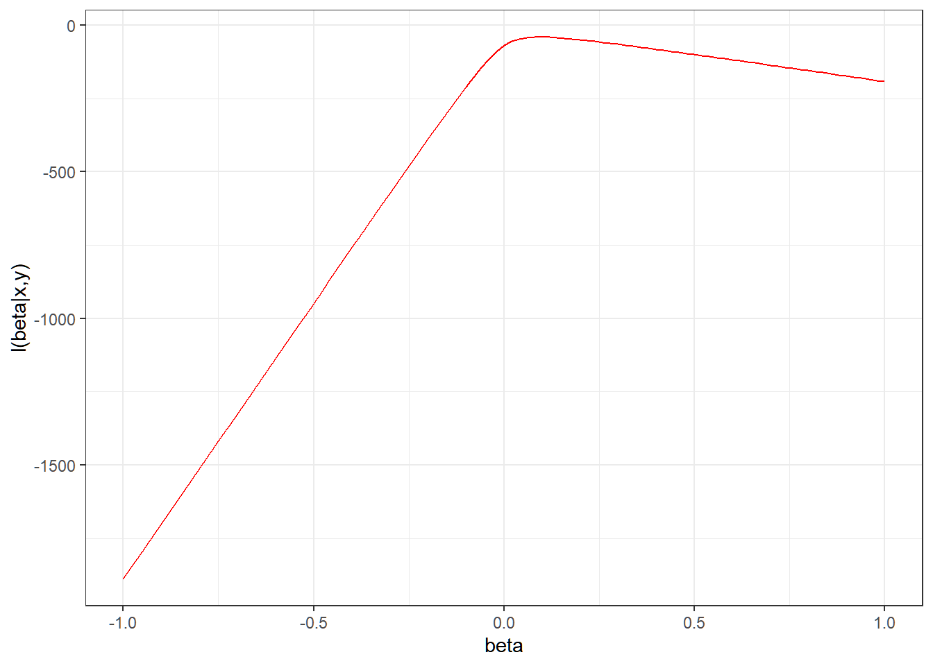
The following is the graph of the log-likelihood function for different values of $\beta$ , given the dataset:

When optimizing, we get the first derivative with respect to $\beta$ :

$\ell'(\beta)=\sum_{i=1}^n \left[ y_i x_i - \left( \frac{1}{1+e^{-\beta x_i}}\cdot x_i\right)\right]\\$

After setting to 0, a closed form solution cannot be obtained for $\hat{\beta}$

The equation is nonlinear and requires an iterative solution, through some optimization algorithm.

There are many methods to find the value of $\beta$ that maximizes this log-likelihood function. Two solutions will be discussed here.

Changing the implementation of a given component can lead to different outcomes further down the change and can even produce completely different outputs. Identical estimates for the parameters in simple linear regression model can be produced by replacing the likelihood principle with the principle of ordinary least squares.

However, changing the principle to produce estimates may produce different statistics at the end.

There is a general principle that Kenneth Lange calls optimization transfer. The basic idea applies to the problem of maximizing a function $f$ .

Definition 3.1 (Optimization Transfer Principle)
The difficult problem of maximizing $f$ is replaced with the simpler problem of maximizing $g$ coupled with iteration (otherwise known as computation).

We want to maximize $f$ , but it is difficult to do so.
We can compute for an approximation of $f$ , call it $g$ , based on local information about $f$ .
Instead of maximizing $f$ , we “transfer” the maximization problem to $g$ and maximize $g$ instead.
We iterate Steps 2 and 3 until convergence.

Note that all of the above applies to minimization problems, because maximizing $f$ is equivalent to minimizing $−f$ .

In statistics we need to optimize many functions, including likelihood functions and generalizations thereof, Bayesian posterior distributions, entropy, and fitness landscapes. These all describe the information content in some observed data. Maximizing these functions can drive inference.

In the succeeding parts, we describe some of the statistical contexts within which optimisation problems arise and a sample of methods for solving them. In particular, we will look into some line search methods — Newton’s method and gradient descent method—to find optimal solutions to statistical problems. Other optimization algorithms will also be introduced.

3.1.1 General Optimization

The general optimization problem can be stated as follows:

Given a function $f:\mathbb{R}^k\rightarrow\mathbb{R}$ , we want to find $\underset{x\in S}{\arg \min}f(x)$ , where $S\subset\mathbb{R}^k$

The general approach in solving this problem that we will discuss is called a line search method. With line search methods, given $f$ and a current estimate $x_t$ of the location of the minimum, we want to:

Choose a direction $p_t$ in $k$ -dimensional space;
Choose a step length $\alpha_t$ in the direction $p_t$
Update the estimate from the current $x_t$ to the next one $x_{t+1}$ , where $x_{t+1} = x_t + \alpha_t p_t$

Until some stopping criterion is satisfied.

The step direction $p_t$

Definition 3.2 $p_t$ , also denoted as $\Delta x_t$ , is a vector in the space $\mathbb{R}^k$ , is called the step direction or search direction.

If $f$ is a univariate function (i.e. only optimizing for one parameter), then $p_t$ is a scalar value.
Sometimes, a unit normalized direction vector $||\Delta x_t||$ is used (for easier interpretability), but not required.

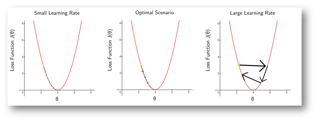
The learning rate $\alpha_t$

Definition 3.3 The $\alpha_t$ is the learning rate or step size of the algorithm. Also called step length or scale factor in other sources. It represents the speed at which an algorithm “learns”.

In general, the learning rate is a tuning parameter in an optimization algorithm that determines the step size at each iteration while moving toward a minimum of a loss function.
The learning rates affects the number of iterations of the algorithm
The range of the learning rate alpha is often $0<\alpha<1$ . In some cases, when alpha is too large, the approximation will not converge (overdampened).
The value may be solved using $\underset{\alpha \geq 0}{\arg \min}f(x_t+ \alpha p_t)$ to get $\alpha_t$ .
- This is called Exact line search.
- This may be used if the cost of searching for $\alpha_t$ is low compared to the cost of computing the search direction itself.
- This step size selection ensures faster convergence.
$\alpha_t$ may be constant, i.e., does not change per iteration: $\alpha_t=\alpha$ .

Clearly then, with line search methods, the two questions one must answer are:

how should we choose the direction $p_t$ ?
how far should we step $\alpha_t$ ?

Almost all line search approaches provide variations on the answers to those two questions.

3.1.2 Steepest Descent

When minimizing $f$ , for a given starting position $x_t$ , the most obvious direction $p_t$ to choose is the direction of its steepest descent, or $-f'(x_t)$ . This is the direction that is orthogonal (or tangential) to the contours of $f$ at some point $x_t$ , and hence is the direction in which $f$ is changing most rapidly at $x_t$ .

Definition 3.4 (Steepest Descent Algorithm)
The updating procedure for a steepest descent algorithm, given the current state $x_t$ is

$x_{t+1} = x_t - \alpha_t f'(x_t)$

If $f$ is a multivariate function then the updating procedure for a vector $\textbf{x}_t$ is

$\textbf{x}_{t+1}=\textbf{x}_t - \alpha_t \nabla f(\textbf{x}_t),$

where $\nabla f$ is the gradient of $f$ .
Much like with optimization problems in calculus, if $f$ is differentiable and convex, a necessary and sufficient condition for a point $x_t$ to be optimal (minimum) is if $f'(x_t)=0$ . Therefore, our algorithm stops if $f'(x_t) \approx 0$ , or very low at some given tolerance value.
Your initial guess $x_0$ may affect whether you will obtain the global optima, while your learning rate $\alpha$ will affect how fast you will obtain an optima (global or local).

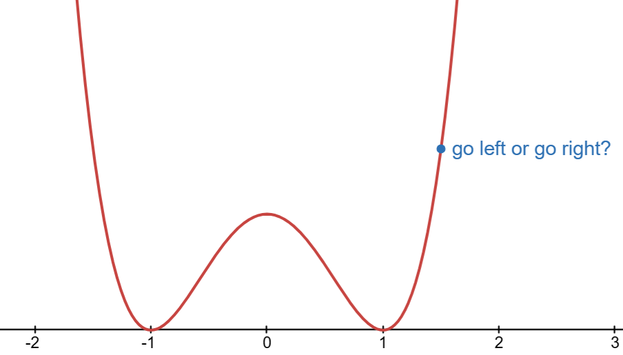
Visualization: $f(x) = x^4-2x^2+1$

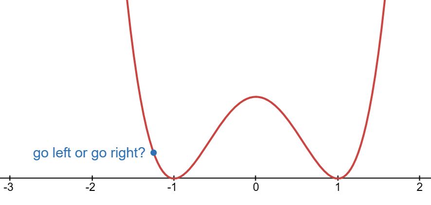
We know that the minimum of $f(x) = x^4-2x^2+1$ is attained at $x=-1$ or $x=1$ .

Let’s try using steepest descent.

Start with an initial guess $x_0=1.5$ .
Show Codes
```
x0 <- 1.5
```
Select direction: $p_t = f'(x_t) = 4x^2 - 4x$
Show Codes
```
f_prime <- function(x){
        return(4*x^3 - 4*x)
}
```
- At $x_t=1.5$ , what is the value of $f'(x_t)$ ?
- When finding the minimum from $x_t=1.5$ , should we go left or go right?
Select learning rate. For this example, we set constant $\alpha = 0.1$
Show Codes
```
alpha <- 0.1
```
Update guess: $x_{t+1}=x_t-\alpha_t p_t$ .
Show Codes
```
x <- x0
x_new  <- x - alpha*f_prime(x)
```

Repeat #4 until convergence: $|x_{t+1}-x_t|\approx0$ .

Show Codes

x <- x0
repeat{
    x_new  <- x - alpha*f_prime(x)
    print(x_new)
    if(abs(x_new - x) < 1e-6) break
    x <- x_new
}

## [1] 0.75
## [1] 0.88125
## [1] 0.9599979
## [1] 0.990105
## [1] 0.9979039
## [1] 0.9995755
## [1] 0.9999149
## [1] 0.999983
## [1] 0.9999966
## [1] 0.9999993
## [1] 0.9999999

Now, consolidating to a function that stores values in each iteration in a dataframe:

Show Codes

f <- function(x){
    x^4 - 2*x^2 + 1 
}
f_prime <- function(x){
    return(4*x^3 - 4*x)
}
steep_f <- function(x0, alpha, tolerance = 1e-6){
    x_vals <- c(x0) # Store x values
    f_vals <- c(f(x0)) # Store function values
    
    x <- x0
    repeat{
        # update
        x_new  <- x - alpha*f_prime(x)
        # store values
        x_vals <- c(x_vals, x_new)
        f_vals <- c(f_vals, f(x_new))
        
        # exit condition
        if(abs(x_new - x) < 1e-6) break
        x <- x_new
    }
    return(data.frame(iter = 0:(length(x_vals)-1), x = x_vals, f = f_vals))
}

Run the algorithm

result <- steep_f(1.5, 0.1, 1e-6)

Problems in Steepest Descent

when certain parameters are highly correlated with each other, the steepest descent algorithm can require many steps to reach the minimum
depending on the starting value, the steepest descent algorithm could take many steps to wind its way towards the minimum
the algorithm may get stuck at a local optimum if there are multiple optima

A Multivariate Example

One can use steepest descent to compute the maximum likelihood estimate of the mean in a multivariate normal density, given a sample of data.

Recall the log-likelihood of Multivariate Normal:

$\begin{align} \log L(\boldsymbol{\mu},\boldsymbol{\Sigma}|\textbf{x}_1,\dots, \textbf{x}_n)&=\log\left(\prod_{i=1}^nf_\textbf{X}(\textbf{x}_i)\right)\\ &=\sum_{i=1}^n\log f_\textbf{X}(\textbf{x}_i) \end{align}$

We know that if we maximize this with respect to $\boldsymbol{\mu}$ , we get $\hat{\boldsymbol{\mu}}=\sum_{i=1}^n\textbf{x}_i$ , but for demonstration, we assume that we don’t know this.

We use the negative log-likelihood since the gradient descent is designed to minimize functions.

Show codes

set.seed(123)
mu <- c(1, 2)
S <- rbind(c(1, .9), c(.9, 1))
x <- MASS::mvrnorm(500, mu, S)
nloglike <- function(mu1, mu2) {
        dmv <- mvtnorm::dmvnorm(x, 
                                c(mu1, mu2), 
                                S, 
                                log = TRUE)
        return(-sum(dmv))
}
nloglike <- Vectorize(nloglike, c("mu1", "mu2"))
nx <- 40
ny <- 40
mu_1 <- seq(-5, 5, len = nx)
mu_2 <- seq(-5, 6, len = ny)
g <- expand.grid(mu_1, mu_2)
nLL <- nloglike(g[, 1], g[, 2])
z <- matrix(nLL, nx, ny, byrow = T)

The following is the graph of the negative log-likelihood function $-L(\boldsymbol{\mu})$ for different values of $\mu_1$ and $\mu_2$ .

The green dot is the MLE for $\boldsymbol{\mu}$ using the derived formula.

However, when the data are highly correlated, as they are in the simulated example, the log-likelihood surface can be difficult to optimize. In such cases, a very narrow ridge develops in the (negative) log-likelihood that can be difficult for the gradient descent algorithm to navigate.

The following implements the gradient descent, where the initial state is at $x_0 = (-5,-2)$ , learning rate $\alpha=1$ , and for $8$ steps only.

Show codes

norm <- function(x) x / sqrt(sum(x^2))
Sinv <- solve(S)  # Not suggested; it solves a system of equations
step1 <- function(mu, alpha = 1) {
        D <- sweep(x, 2, mu, "-")
        score <- colSums(D) %>% norm
        mu + alpha * drop(Sinv %*% score)
}
steep <- function(mu, n = 10, ...) {
        results <- vector("list", length = n)
        for(i in seq_len(n)) {
                results[[i]] <- step1(mu, ...)
                mu <- results[[i]]
        }
        results
}
m <- do.call("rbind", steep(c(-5, -2), 8))
m <- rbind(c(-5, -2), m)

We can see that the path of the algorithm is rather winding as it traverses the narrow valley.

Now, we have fixed the step-length in this case, which is probably not optimal. However, one can still see that the algorithm has some difficulty navigating the surface because the direction of steepest descent does not take one directly towards the minimum ever.

We can also adjust the learning rate $\alpha$ to 0.25 and increase the number of iterations from 8 to 60.

Show codes

m <- do.call("rbind", steep(c(-5, -2), 60, alpha=0.25))
m <- rbind(c(-5, -2), m)

We can also change the initial guess to $x_0=(0,0)$

Show codes

m <- do.call("rbind", steep(c(0, 0), 13, alpha=0.25))
m <- rbind(c(0, 0), m)

3.1.3 Newton’s Method

Definition 3.5 (Newton Step)
The updating procedure for the Newton’s Method is

$x_{t+1} = x_t - \frac{f'(x_t)}{f''(x_t)}$

If $f$ is a multivariate function then the updating procedure for a vector $\textbf{x}_t$ is

$\textbf{x}_{t+1} = \textbf{x}_{t} -\nabla^2f(\textbf{x}_t)^{-1}\nabla f(\textbf{x}_t)$
Newton’s method has a “natural” step length $\alpha$ of 1.

Proof: Univariate case

GOAL: For a given value $x_t$ and function $f$ , find the value of the step $p_t$ such that $f(x_t+p_t)$ will be at the optimum.

If $f$ is hard to optimize, we can first approximate $f$ with a quadratic polynomial, then perform optimization on this new function.

For some small $p_t$ , the second-order Taylor series expansion of $f$ around $x_t$ is given by

$f(x_t + p_t) \approx f(x_t)+p_t f'(x_t)+\frac{1}{2}p_t^2f''(x_t)$

Obtain the first derivative of $f(x_t +p_t)$ respect to $p_t$ :

$\begin{align} \frac{d}{dp_t}f(x_t+p_t) & \approx \frac{d}{dp_t}\left[f(x_t)+p_t f'(x_t)+\frac{1}{2}p_t ^2f''(x_t)\right] \\ &= f'(x_t) + p_t f''(x_t) \end{align}$

Now equating to $0$ and solving for $p_t$ , we get:

$p_t = -\frac{f'(x_t)}{f''(x_t)}$

Note that this logic states that the next iterate $x_{t+1}$ is defined to be able to minimize the quadratic approximation in $p_t$ , such that $x_{t+1}=x_t + p_t$ .

And thus, $x_{t+1}=x_t-\frac{f'(x_t)}{f''(x_t)}$ $\blacksquare$

Newton’s method makes a quadratic approximation to the target function $f$ at each step of the algorithm. This follows the “optimization transfer” principle mentioned earlier, whereby we take a complex function $f$ , replace it with a simpler function $g$ that is easier to optimize, and then optimize the simpler function repeatedly until convergence to the solution.

Direction of the step

Recall that if the second derivative of $f$ is positive, then we are looking at a minimum, implying that $-\frac{f'(x_t)}{f''(x_t)}$ is a descent direction.
If $f''$ is negative, then we are looking for a maximum, i.e. $-\frac{f'(x_t)}{f''(x_t)}$ is an ascent direction.

This further implies that Newton’s method is not restricted to finding the minimum of a function only. This can be also used for finding the maximum (i.e. the function is concave)

Steepest Descent vs Newton’s Method

When we look at the update statements, we would see that the learning rate in Newton’s method is $\alpha_t=\frac{1}{f''(x_t)}$ . The idea is that if slope changes too quickly (high $|f''(x_t)|$ ), learning slows down; if it changes too slowly (low $|f''(x_t)|$ ), learning speeds up.

Method	Steepest Descent	Newton’s Method
Update Statement	$x_{t+1} =x_t\alpha_t f'(x_t)$	$x_{t+1} =x_t- \frac{f'(x_t)}{f''(x_t)}$
Learning Rate	Requires a specific learning rate: $a_t$	Does not require a specific learning rate; the learning rate is a function of the 2nd derivative $\frac{1}{f''(x_t)}$
Derivation	Requires the first derivative only	Requires both first and second derivative
Convergence	May converge slowly if we need more iterations to reach the minimum	May converge faster especially if the function is quadratic in nature
Division by 0	No problem in terms of division by 0	Might be unstable if $f''(x_t)=0$ (e.g. $x_t$ is an inflection point)

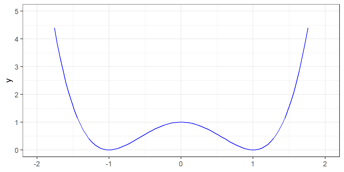
Visualization: $f(x) = x^4-6x^2+9$

$f(x) = x^4 - 6x^2 + 9$
$f'(x) = 4x^3-12x$
$f''(x)=12x^2-12$
$x_{t+1}=x_t-\frac{4x^3-6x}{12x^2-6}$

f <- function(x){
    x^4 - 6*x^2 + 9
}

f_prime <- function(x){
    return(4*x^3 - 12*x)
}

f_double_prime <- function(x){
    return(12*x^2 - 12)
}

newton_f <- function(x0, tol){
    
    # storing values
    x_val <- c(x0)
    
    x <- x0
    repeat{
        x_new <- x-f_prime(x)/f_double_prime(x)
        x_val <- c(x_val, x_new)
        if(abs(x_new - x) < tol) break
        x <- x_new
    }
    
    f_val <- f(x_val)
    iter  <- 0:(length(x_val)-1)
    return(data.frame(iter, 
                      x = x_val, 
                      f = f_val))
}

result2 <- newton_f(1.5, 1e-6)

$f(x)$ is at minimum when $x=$ 1.7320508

Now, note that $x=1$ is an inflection point. The Newton’s algorithm will have a problem in finding the optima if this is your starting point, since it does not know if it is finding a maximum or minimum.

# this will show an error
newton_f(x0 = 1, tol = 1e-6)

Example 1: estimating $\beta$ in the logistic regression model

Recall the log-likelihood function for $\beta$ in the logistic regression model:

$\ell(\beta)=\sum_{i=1}^n [y_i\beta x_i-\log(1+e^{\beta x_i})]$

Given the dataset $(y_1,x_1), (y_2,x_2),...,(y_{100}, x_{100})$

binary_data

ABCDEFGHIJ0123456789

y <dbl>	x <dbl>
1	31.3680213
1	42.6021356
1	22.0080756
1	-14.5386236
1	-4.2297142
0	26.6194716
1	17.9593872
1	0.9560583
0	-26.2415985
1	5.3078376

the following is the plot of the likelihood function for different values of $\beta$

logreg_plot

The Newton equation to estimate optimal $\beta$ is given as

$\beta_{t+1} = \beta_t - \frac{l'(\beta_t)}{l''(\beta_t)}$

The first and second order derivatives of $\ell(\beta)$ are

$\ell'(\beta)=\sum_{i=1}^n \left[ x_i \left(y_i - \pi(x_i,\beta)\right)\right]\\ \ell''(\beta) = -\sum_{i=1}^n \left(x_i^2 \pi(x_i,\beta)(1-\pi(x_i,\beta))\right)$

where

$\pi(x_i,\beta) = \frac{e^{\beta x_i}}{1+e^{\beta x_i}}$

The following R codes implement Newton’s Method to estimate the $\beta$ in the logistic regression model:

newton_logistic <- function(x, y, beta_init = 0, tol = 1e-6, max_iter = 100) {
  beta <- beta_init
  for (iter in 1:max_iter) {
    # Compute the probability π(x) = exp(βx) / (1 + exp(βx))
    pi_x <- exp(beta * x) / (1 + exp(beta * x))
    
    # Compute gradient (first derivative of log-likelihood)
    gradient <- sum(x * (y - pi_x))
    
    # Compute Hessian (second derivative of log-likelihood)
    hessian <- -sum(x^2 * pi_x * (1 - pi_x))
    
    # Update beta using Newton-Raphson method
    beta_new <- beta - gradient / hessian
    
    # Check for convergence
    if (abs(beta_new - beta) < tol) {
      return(beta_new)
    }
    
    beta <- beta_new
  }
  
  warning("Newton's Method did not converge within the max iterations")
  return(beta)
}

betahat <- newton_logistic(binary_data$x, binary_data$y)
betahat

## [1] 0.09470147

logreg_plot + 
    geom_vline(xintercept = betahat)+
    geom_hline(yintercept = loglik_lgstc(betahat,
                                         binary_data$x,
                                         binary_data$y),
               linetype = "dashed")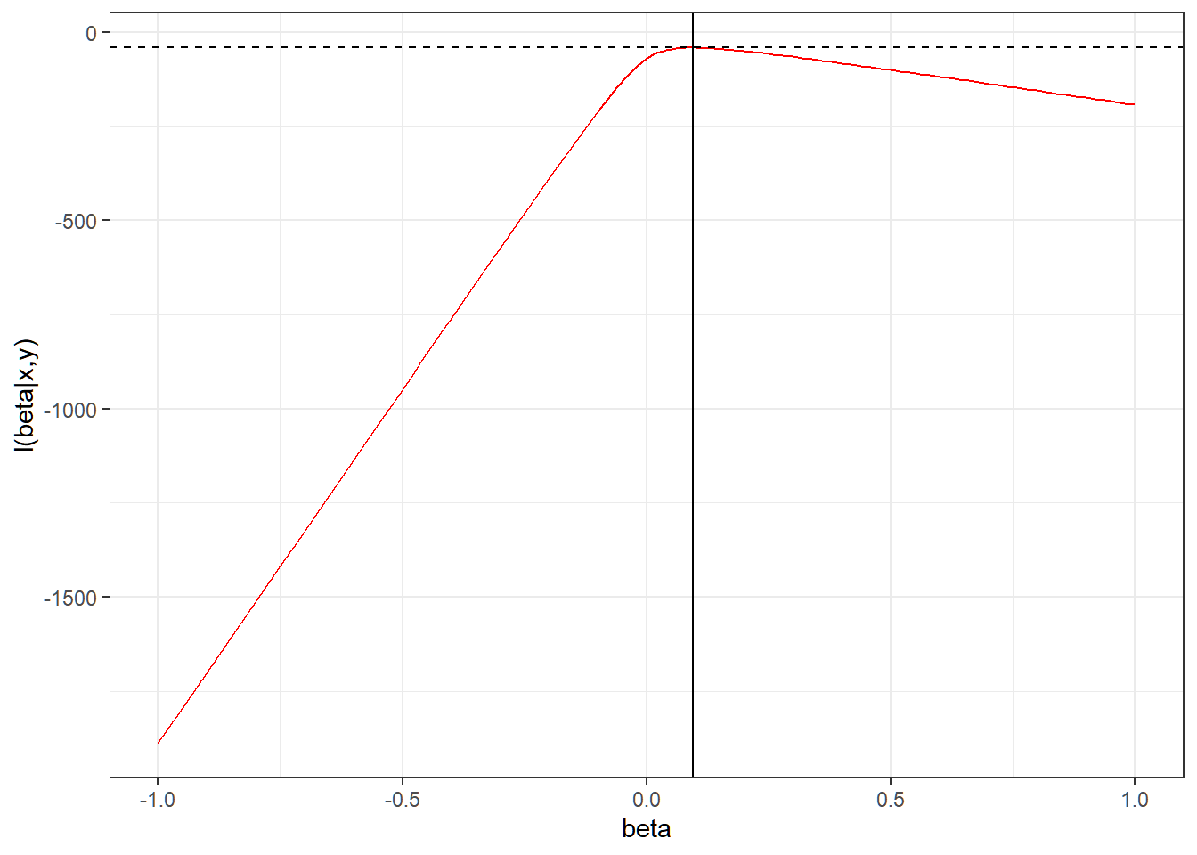

Example 2: Multivariate Case

Recall the updating procedure for optimizing a multivariate function:

$\textbf{x}_{t+1} = \textbf{x}_{t} -\nabla^2f(\textbf{x}_t)^{-1}\nabla f(\textbf{x}_t)$

where $\nabla^2f(\textbf{x}_t)^{-1}$ is the inverse of the Hessian matrix, and $\nabla f(\textbf{x}_t)$ is the Gradient.

The following is a general function for implementing Newton’s method:

newton_optim <- function(f, grad_f, hess_f, x0, tol = 1e-6, max_iter = 100) {
  x <- x0
  for (i in 1:max_iter) {
    g <- grad_f(x)
    H <- hess_f(x)
    
    # Solve H * p = -g for p
    p <- tryCatch(solve(H, -g), error = function(e) {
      warning("Hessian is not invertible.")
      return(rep(NA, length(x)))
    })
    
    if (any(is.na(p))) break
    
    x_new <- x + p
    
    if (sqrt(sum((x_new - x)^2)) < tol) {
      message("Converged in ", i, " iterations.")
      return(x_new)
    }
    
    x <- x_new
  }
  warning("Maximum number of iterations reached without convergence.")
  return(x)
}

For example, we want to find the value of $\textbf{x} = [x_1, x_2]'$ that optimize the following function:

$f(x_1,y_2) = 100(x_2-x_1^2)^2+(1-x_1)^2$

This is called the Rosenbrock Function.

The gradient is given by:

$\nabla f(x_1,x_2) = \begin{bmatrix} \frac{\partial f}{\partial x_1} \\ \frac{\partial f}{\partial x_2} \end{bmatrix} =\begin{bmatrix} -400x(x_2-x_1^2) - 2(1-x_1) \\ 200(x_2-x_1^2)\end{bmatrix}$

and the Hessian matrix is given by

$\nabla^2f(x_1,x_2) = \begin{bmatrix} \frac{\partial^2 f}{\partial x_1^2} & \frac{\partial^2 f}{\partial x_1 \partial x_2} \\ \frac{\partial^2 f}{\partial x_2 \partial x_21} & \frac{\partial^2 f}{\partial x_2^2} \end{bmatrix}= \begin{bmatrix} 1200x_1^2-400x_2+2 & 400x_1 \\ -400x_1 & 200 \end{bmatrix}$

Now, using Newton’s method:

rosenbrock <- function(x) {
  100 * (x[2] - x[1]^2)^2 + (1 - x[1])^2
}

grad_rosenbrock <- function(x) {
  c(
    -400 * x[1] * (x[2] - x[1]^2) - 2 * (1 - x[1]),
    200 * (x[2] - x[1]^2)
  )
}

hess_rosenbrock <- function(x) {
  matrix(c(
    1200 * x[1]^2 - 400 * x[2] + 2,
    -400 * x[1],
    -400 * x[1],
    200
  ), nrow = 2, byrow = TRUE)
}

# Start at initial point
x0 <- c(-1.2, 1)

result <- newton_optim(rosenbrock, grad_rosenbrock, hess_rosenbrock, x0)

## Converged in 7 iterations.

print(result)

## [1] 1 1

3.1.4 Overview of other optimization algorithms

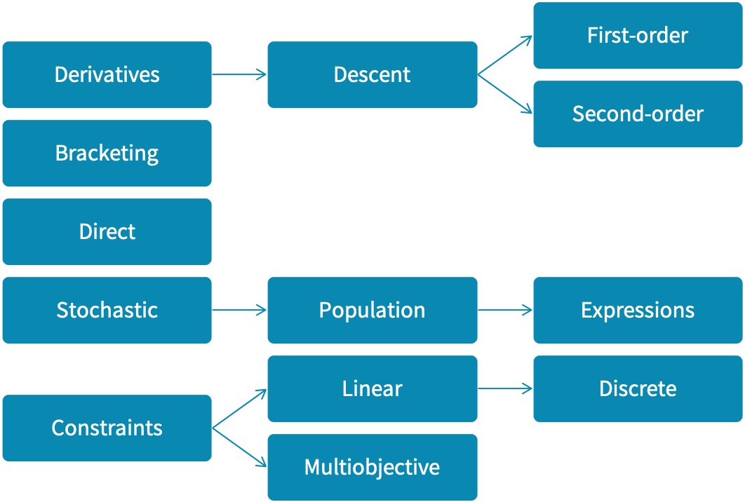
Optimization algorithms fall into several categories:

Derivative-based methods like steepest descent and Newton’s method use derivatives to guide the search. When derivatives are unavailable, we estimate them numerically or with automatic differentiation.
Bracketing methods iteratively narrow an interval containing a local minimum, sometimes using a function’s Lipschitz constant. These methods are often subroutines in optimization.
Direct search methods avoid gradients, using line search, pattern search, or adaptive simplex techniques to explore the design space.
Stochastic methods incorporate randomness, sometimes refining gradient-based or direct search techniques, or learning probability distributions over the search space.
Penalty-based methods introduce constraints through penalty functions.

Exercise: Multiple logistic regression

Again, in logistic regression, we want to model the probability of success of $Y_i$ for some given input $\textbf{x}_i$ .

Suppose $Y_i$ is a binary random variable, $\textbf{x}_i$ is a $1\times k$ vector of observed values of the regressors for observation $i$ , and $\boldsymbol{\beta}$ is a $k \times 1$ vector of parameters, we have the following model for the probability of success of $Y$ .

$P(Y_i=1|\textbf{x}_i)=\pi(\textbf{x}_i) = \frac{e^{\textbf{x}_i\boldsymbol{\beta}}}{1+e^{\textbf{x}_i\boldsymbol{\beta}}}$

The log-likelihood of the logistic model, given $n$ observations, is given by

$\ell(\boldsymbol{\beta}| \textbf{y}, \textbf{X})=\sum_{i=1}^n\left[-\log(1+\exp(\textbf{x}_i\boldsymbol{\beta}))+y_i\textbf{x}_i\boldsymbol{\beta}\right]$

The maximum likelihood estimator $\hat{\boldsymbol{\beta}}$ of the parameter $\boldsymbol{\beta}$ solves

$\hat{\boldsymbol{\beta}}=\underset{\boldsymbol{\beta}}{\arg\max}\left\{\ell(\boldsymbol{\beta}|\textbf{y},\textbf{X}) \right\}$

But again, the solution to this optimization problem has no closed form, and thus requires an iterative solution, such as the Newton’s method.

For your convenience, here are the first and second derivatives of the log-likelihood function:

The first derivatives of the log-likelihood with respect to the parameter vector $\boldsymbol{\beta}$ , or the “score vector” is

$\nabla_\boldsymbol{\beta}\ell(\boldsymbol{\beta}| y, X)=\sum_{i=1}^n \left[\textbf{x}_i \left(y_i - \pi(\textbf{x}_i)\right)\right]\\$
The second derivative of the log-likelihood, called the Hessian Matrix, can be defined as:

$\nabla_{\beta\beta}\ell(\boldsymbol{\beta}|\textbf{y},\textbf{X}) = -\sum_{i=1}^n \left(\textbf{x}_i'\textbf{x}_i \pi(\textbf{x}_i)(1-\pi(\textbf{x}_i))\right)$

TASK: Create a function log_reg that implements Newton’s method to estimate the coefficient vector $\boldsymbol{\beta}$

INPUT parameters:

the response vector y containing 1s and 0s only
the design matrix X, where the first column is a column of 1s, for the estimation of the “bias term” (related with the intercept in linear regression).
the initial values for the parameter vector beta_init = rep(0,ncol(X)). Default value is a vector of zeroes $(0,0,...,0)$ .
The tolerance tol = 1e-6, which is the exit condition for the Newton’s algorithm.
The maximum number of iterations: max_iter = 10. Show a message if no convergence can be seen after the maximum number of iterations that was set.

Apply the function on the data that can be found on logreg_data.csv. Feel free to create vectors or matrices from this dataframe prior to inputting it to your function.

OUTPUT: a vector of the estimated beta