2.3 Optimizing Program Performance

In the this digital age, datasets are getting larger, and extracting insights from them in the shortest possible time is of growing demand

Optimizing program performance enables the handling of larger datasets and more computationally intensive tasks.

The following introduces some techniques to optimize your program performance.

2.3.1 Organizing Code

There are two traps that are easy to fall into when trying to make your code faster:

Writing faster but incorrect code.
Writing code that you think is faster but is actually no better.

Writing well-structured code improves readability, maintainability, and performance.

Key principles include:

Modularization: Break down code into reusable functions.
Avoiding redundant calculations: Store intermediate results instead of recomputing them.
Profiling: Use profvis() or Rprof() to identify bottlenecks.

2.3.2 Preallocating Memory

Avoid growing objects dynamically inside loops, as it leads to memory reallocation overhead.

A good rule of thumb is to compare your objects before and after a loop; have they increased in length?

In R, you don’t have to explicitly allocate memory before you use it.
You can pre-allocate memory by setting the length, nrow, ncol, or dim attributes for an object.
You should also consider pre-allocating memory for data frames and lists.

Example

We will create a function that generates a vector of integers from 1 up to $n$ .
Without pre-allocation (slow)
method1 <- function(n) {
    vec <- c()
    for (i in 1:n) {
        vec <- c(vec, i)  # Reallocates memory every iteration
    }
    return(vec)
}
This creates an empty vector and gradually increases (or grows) the length of the vector.
With pre-allocation (fast)
method2 <- function(n) {
  vec <- numeric(n)
  for (i in 1:n) {
    vec[i] <- i
  }
  return(vec)
}
This creates an object of with pre-defined length and then changes the values in the object by indexing.
directly creating the final object
method3 <- function(n) {seq_len(n)}
All these methods yield the same outcome yet differ in terms of efficiency.

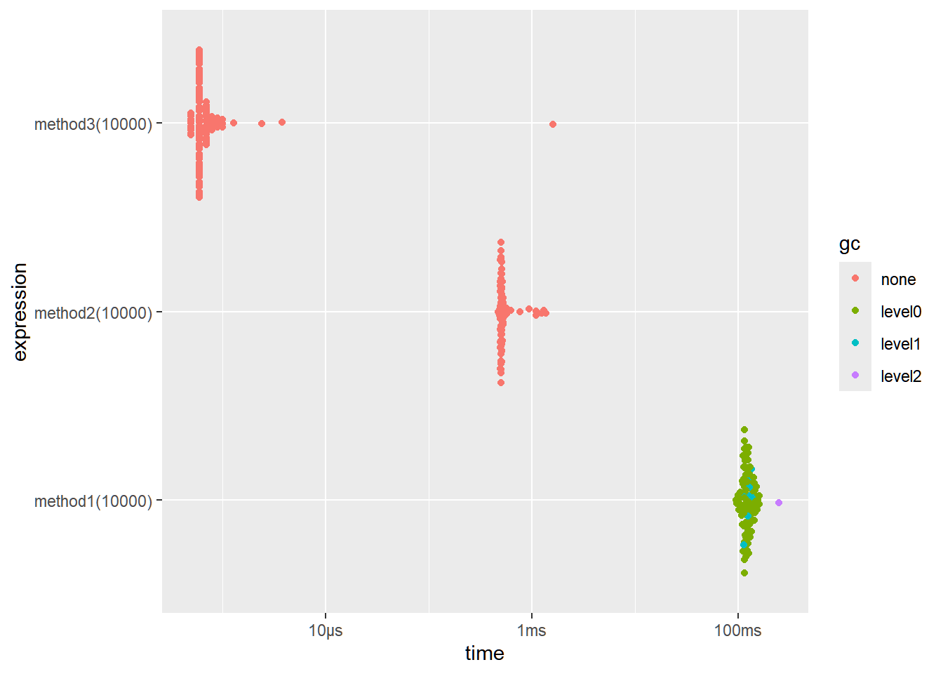
If we try to compare using microbenchmarking:
result <- bench::mark(
  method1(1e4),
  method2(1e4),
  method3(1e4),
  iterations = 100, time_unit = "ms"
)
result[c("expression", "min", "median", "itr/sec", "n_gc")]
ABCDEFGHIJ0123456789
expression
<bnch_xpr>
min
<dbl>
median
<dbl>
itr/sec
<dbl>
<bnch_xpr> 94.9564 121.24500 8.047288
<bnch_xpr> 0.4704 0.50785 1810.957743
<bnch_xpr> 0.0005 0.00060 60067.275347
3 rows
plot(result)

expression <bnch_xpr>	min <dbl>	median <dbl>	itr/sec <dbl>
<bnch_xpr>	94.9564	121.24500	8.047288
<bnch_xpr>	0.4704	0.50785	1810.957743
<bnch_xpr>	0.0005	0.00060	60067.275347

2.3.3 Vectorizing

Vectorization in R leverages optimized C-based operations instead of loops, significantly improving speed.

Many R functions are vectorized, that is the function’s inputs and/or outputs naturally work with vectors, reducing the number of function calls required. For example, the code

x <- runif(n) + 1

performs two vectorized operations. First runif() returns n random numbers. Second, we add 1 to each element of the vector. In general, it is a good idea to exploit vectorized functions.

Example

Consider this piece of R code that calculates the square of each element of x:

# Using a loop (slow)
square_loop <- function(x) {
  res <- numeric(length(x))
  for (i in seq_along(x)) {
    res[i] <- x[i]^2
  }
  return(res)
}

How can we vectorize this?

Answer

Straightforward, using the operation x^2

# Vectorized version (fast)
square_vec <- function(x) {
  return(x^2)
}

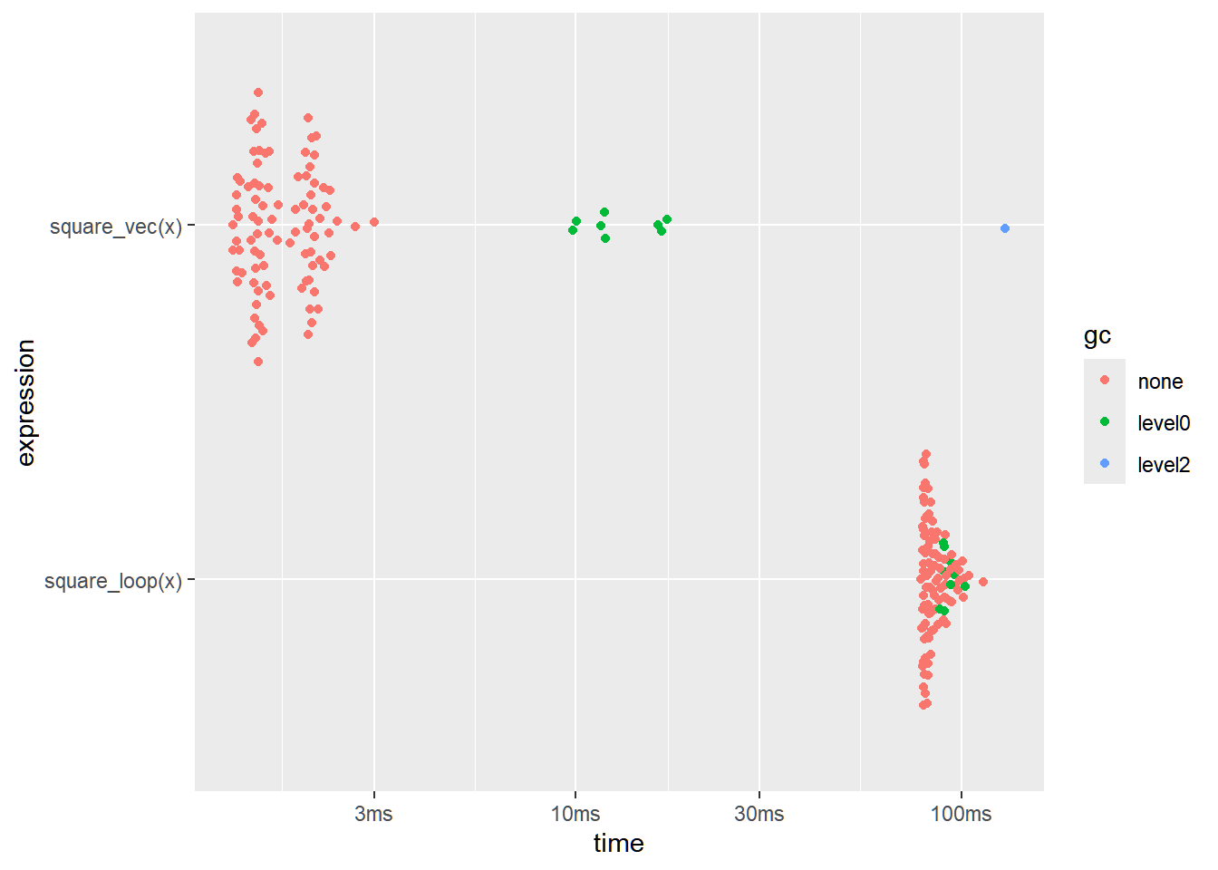
For a quick test, we have the following benchmarking:

x <- 1:1000000
result <- bench::mark(square_loop(x), 
                      square_vec(x),
                      iterations = 100, 
                      time_unit = "ms"
                      )
result[c("expression", "min", "median", "itr/sec")]

ABCDEFGHIJ0123456789

expression <bnch_xpr>	min <dbl>	median <dbl>	itr/sec <dbl>
<bnch_xpr>	78.3229	83.1027	11.68007
<bnch_xpr>	1.2912	1.5997	569.75633

plot(result)

Note: There are three levels of collections.

Level 0 collects only the youngest generation, level 1 collects the two youngest generations and level 2 collects all generations.
After 20 level-0 collections the next collection is at level 1,
and after 5 level-1 collections at level 2.
Further, if a level-n collection fails to provide 20% free space (for each of nodes and the vector heap), the next collection will be at level $n+1$ .
The R-level function gc() performs a level-2 collection.

Writing code this way has a number of benefits.

It’s faster. When $n=10^6$ , the R way is about four times faster.
It’s neater.
It doesn’t contain a bug when x is of length 0.

Important note:

The slowdown isn’t due to the for loop. Instead, it’s because there are many more function calls.
So instead of going through a loop and performing many function calls, it’s better if we can exploit vectorized operations in R.

2.3.4 Using Matrix Operations

Another reason why matrix operations is taught is that they are sometimes more efficient when applied in programs.

This is an extension of vectorizing.

For example, using nested loops for matrix multiplication

A <- matrix(rnorm(10000), 100, 100)
B <- matrix(rnorm(10000), 100, 100)

mat_mul <- function(X,Y){
    Z <- matrix(0, 100, 100)
    for (i in 1:100) {
      for (j in 1:100) {
        for (k in 1:100) {
          Z[i, j] <- Z[i, j] + X[i, k] * Y[k, j]  # Very slow
        }
      }
    }
    return(Z)
}

bench::mark(mat_mul(A,B), A%*%B, 
            time_unit = "us")

ABCDEFGHIJ0123456789

expression <bnch_xpr>	min <dbl>	median <dbl>	itr/sec <dbl>	mem_alloc <bnch_byt>	gc/sec <dbl>
<bnch_xpr>	168705.1	175928.8	5.681797	124.96094KB	0
<bnch_xpr>	491.4	510.6	1815.551922	78.17188KB	0

WARNING: Problems in Precision

However, be careful for possible rounding off errors due to floating-point arithmetic.

This is expected when performing matrix operations like Jbar %*% mat, since matrix multiplication involves multiple floating-point operations.

Suppose we have the following dataset
X <- data.frame(x1 = c(2,3,4,5,6),
                  x2 = c(7,9,11,13,15),
                  x3 = c(1,3,6,9,11))
X
ABCDEFGHIJ0123456789
x1
<dbl>
x2
<dbl>
x3
<dbl>
2 7 1
3 9 3
4 11 6
5 13 9
6 15 11
5 rows

You want to subtract each element from the mean of each column. In other words, you are “centering” this dataset.

You may premultiply the centering matrix $\textbf{I}-\bar{\textbf{J}}$ to the matrix.
I    <- diag(1, nrow = 5)
Jbar <- matrix(rep(1, 5^2), nrow = 5)/5
I
Jbar
##      [,1] [,2] [,3] [,4] [,5]
## [1,]    1    0    0    0    0
## [2,]    0    1    0    0    0
## [3,]    0    0    1    0    0
## [4,]    0    0    0    1    0
## [5,]    0    0    0    0    1
##      [,1] [,2] [,3] [,4] [,5]
## [1,]  0.2  0.2  0.2  0.2  0.2
## [2,]  0.2  0.2  0.2  0.2  0.2
## [3,]  0.2  0.2  0.2  0.2  0.2
## [4,]  0.2  0.2  0.2  0.2  0.2
## [5,]  0.2  0.2  0.2  0.2  0.2
Now obtaining $(\textbf{I}-\bar{\textbf{J}})\textbf{X}$
(I - Jbar) %*% as.matrix(X)
##      x1            x2            x3
## [1,] -2 -4.000000e+00 -5.000000e+00
## [2,] -1 -2.000000e+00 -3.000000e+00
## [3,]  0  4.440892e-16  8.881784e-16
## [4,]  1  2.000000e+00  3.000000e+00
## [5,]  2  4.000000e+00  5.000000e+00
This happened because the centering matrix $(\textbf{I}-\bar{\textbf{J}})$ contains decimal values, which may not represent the exact values they want to represent, which then propagates after the matrix multiplication with $\textbf{X}$

As an alternative, you may use the following:

$\textbf{X}-\bar{\textbf{J}}\textbf{X}$
(as.matrix(X) - Jbar%*%as.matrix(X))
##      x1 x2 x3
## [1,] -2 -4 -5
## [2,] -1 -2 -3
## [3,]  0  0  0
## [4,]  1  2  3
## [5,]  2  4  5
With this,

$\bar{\textbf{J}}\textbf{X}$ is computed first, which is just a matrix of column means.

Subtracting this from $\textbf{X}$ only involves basic subtraction.

Fewer floating-point operations = less accumulation of error.

x1 <dbl>	x2 <dbl>	x3 <dbl>
2	7	1
3	9	3
4	11	6
5	13	9
6	15	11

2.3.5 Doing as little as possible

The easiest way to make a function faster is to let it do less work. One way to do that is use a function tailored to a more specific type of input or output, or to a more specific problem.

For example:

rowSums(), colSums(), rowMeans(), and colMeans() are faster than equivalent invocations that use apply() because they are vectorised.
Example
Suppose we have the matrix $\textbf{Y}$
```
Y <- matrix(1:500, ncol = 5)
```
Let’s try getting the sum of each column of Y in two ways:
- Using sum with apply
  apply(Y,2,sum)
```
## [1]  5050 15050 25050 35050 45050
```
- The colSums function
  colSums(Y)
```
## [1]  5050 15050 25050 35050 45050
```
Benchmarking the two functions, we have:
```
bench::mark(apply(Y, 2, sum),
            colSums(Y),
            check=T,
            iterations = 100)
```
ABCDEFGHIJ0123456789
expression
<bnch_xpr>
min
<bench_tm>
median
<bench_tm>
itr/sec
<dbl>
mem_alloc
<bnch_byt>
gc/sec
<dbl>
<bnch_xpr> 34.9µs 38.5µs 23709.04 6.375KB 0
<bnch_xpr> 4.5µs 5µs 190439.92 0B 0
2 rows

The performance of vector operations, matrix operations, and certain specialized functions may vary. When developing a program, it is advisable to experiment to determine the most efficient approach for your specific case.
vapply() is faster than sapply() because it pre-specifies the output type through its parameter FUN.VALUE.
Example
```
numbers <- list(a = 1:1000, b = 1001:2000, c = 2001:3000)
```
```
sapply(numbers, sum)
```
```
##       a       b       c 
##  500500 1500500 2500500
```
```
vapply(numbers, sum, numeric(1))
```
```
##       a       b       c 
##  500500 1500500 2500500
```
```
bench::mark(sapply(numbers, sum),
            vapply(numbers, sum, numeric(1))
)
```
ABCDEFGHIJ0123456789
expression
<bnch_xpr>
min
<bench_tm>
median
<bench_tm>
itr/sec
<dbl>
mem_alloc
<bnch_byt>
gc/sec
<dbl>
<bnch_xpr> 20.5µs 21.9µs 42603.91 0B 8.522486
<bnch_xpr> 8.8µs 9.7µs 93825.83 0B 9.383521
2 rows

Explanation:
- sapply(): Returns a vector or matrix, depending on the result of the applied function. It does not require you to specify the output type.
- vapply(): Requires you to specify the output type, which makes it more efficient since it avoids guessing the result structure.
Some functions coerce their inputs into a specific type. If your input is not the right type, the function has to do extra work. Instead, look for a function that works with your data as it is, or consider changing the way you store your data.
Other functions will do less work if you give them more information about the problem.
- read.csv(): specify known column types with colClasses. (Also consider switching to readr::read_csv() or data.table::fread() which are considerably faster than read.csv().)
- factor(): specify known levels with levels.
- cut(): don’t generate labels with labels = FALSE if you don’t need them, or, even better, use findInterval() as mentioned in the “see also” section of the documentation.
- unlist(x, use.names = FALSE) is much faster than unlist(x).
- interaction(): if you only need combinations that exist in the data, use drop = TRUE.

expression <bnch_xpr>	min <bench_tm>	median <bench_tm>	itr/sec <dbl>	mem_alloc <bnch_byt>	gc/sec <dbl>
<bnch_xpr>	34.9µs	38.5µs	23709.04	6.375KB	0
<bnch_xpr>	4.5µs	5µs	190439.92	0B	0

expression <bnch_xpr>	min <bench_tm>	median <bench_tm>	itr/sec <dbl>	mem_alloc <bnch_byt>	gc/sec <dbl>
<bnch_xpr>	20.5µs	21.9µs	42603.91	0B	8.522486
<bnch_xpr>	8.8µs	9.7µs	93825.83	0B	9.383521

The best way to solve this problem is to read widely so that you can build up your own vocabulary over time.

Record all solutions that you find, not just those that immediately appear to be faster. Some solutions might be slower initially, but end up being faster because they’re easier to optimize.

2.3.6 Parallel Computing

Parallel computing is an essential tool for statisticians working with large datasets or complex models, offering a way to split computations into smaller tasks that can be executed simultaneously.

By leveraging multiple processors or cores, parallel computing can significantly reduce computation time and improve efficiency.

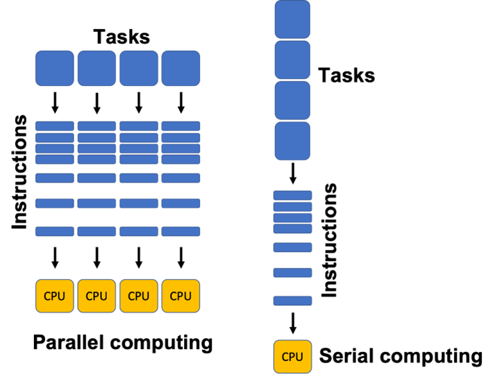
Source: https://pythonnumericalmethods.berkeley.edu/notebooks/chapter13.01-Parallel-Computing-Basics.html

Definition 2.4
Parallel computing uses multiple computer cores to attack several operations at once. Unlike serial computing, parallel architecture can break down a job into its component parts and multi-task them. Parallel computer systems are well suited to modeling and simulating real-world phenomena.

Key Concepts

Parallelism: The simultaneous execution of multiple tasks.
Shared Memory vs. Distributed Memory: Shared memory systems allow processors to access the same memory, while distributed memory systems use separate memories and communicate over a network.
Multithreading: Running multiple threads within a single process concurrently.

Parallel Computing in R

R offers several tools for parallel computing, including the parallel package.

library(parallel)

detectCores() # for my device

## [1] 16

Note that the value returned by detectCores() is dependent on the operating system and hardware of your machine.

The most used parallel applications are parallelized replacements of lapply(), sapply() and apply() (i.e., parLapply , parApply, and parSapply)

We will have examples of this in Section 3.3.

To those interested about learning more about parallel computing in R, I suggest you read Parallel Processing in R by Josh Errickson.

We will not be discussing this in detail since this would be better to be discussed in another course.

2.3.7 Compiling Code

Compilation is the process of translating R code into byte-code that can be executed more efficiently.

The compiler package, introduced in R 2.13.0, compiles R functions into byte-code for faster execution by reducing interpretation overhead.

Since R 2.14.0, base R functions like mean() are pre-compiled by default.

getFunction("mean")

## function (x, ...) 
## UseMethod("mean")
## <bytecode: 0x0000023530f3f7e0>
## <environment: namespace:base>

The third line contains the bytecode of the function. This means that the compiler package has translated the R function into another language that can be interpreted by a very fast interpreter. Amazingly the compiler package is almost entirely pure R, with just a few C support routines.

Compiling your own function

The compiler package, introduced in R 2.13.0, enables this by reducing interpretation overhead. Since R 2.14.0, base R functions like mean() are pre-compiled by default.

The compiler package comes with R, so we just need to load the package in the usual way.

library(compiler)

To demonstrate, we create an inefficient function for calculating the mean. This function takes in a vector, calculates the length and then updates the m variable.

mean_r <- function(x) {
  m <- 0
  n <- length(x)
  for (i in seq_len(n))
    m <- m + x[i] / n
  m
}

This is clearly a bad function and we should just use the mean() function, but it’s a useful comparison.

Compiling the function is straightforward, using the cmpfun function.

cmp_mean_r <- cmpfun(mean_r)

x <- runif(100)
mean_r(x)
cmp_mean_r(x)

## [1] 0.4937434
## [1] 0.4937434

However, in some cases, using bench::mark() may show that an uncompiled function runs faster. This can happen because compiling introduces additional overhead, especially for very short functions where the compilation time outweighs the performance gains.

The benefits of compilation are more noticeable in complex functions that involve many computations or loops.

Exercises

Consider this piece of R code:
```
log_sum1 <- function(x){
  log_sum <- 0
  for (i in 1:length(x)){
    log_sum <- log_sum + log(x[i])
  }
  return(log_sum)
}
```
Create another function log_sum2 that shows the same outputs, but uses vectorization.

Compare results by running this chunk:
```
bench::mark(
  log_sum1(x),
  log_sum2(x),
  iterations = 100, time_unit = "ms"
)
```
Also, check its median relative performance by computing

$\text{relative performance of log_sum1} = \frac{\text{median run time of log_sum1 }}{\text{median run time of log_sum2}}$
The following codes create a growing dataframe per iteration. It has two columns, a, which contains integers from 1 to n, and b which contains the square of the integers from 1 to n.
```
no_prealloc_df <- function(n) {
    df <- data.frame()
    for (i in 1:n) {
        df <- rbind(df, data.frame(a = i, b = i^2))
    }
    return(df)
}
```
```
no_prealloc_df(5)
```
ABCDEFGHIJ0123456789
a
<int>
b
<dbl>
1 1
2 4
3 9
4 16
5 25
5 rows

Create a new function that creates the same output above, but with pre-allocation.

You may initialize a dataframe with zeroes using the following:
```
data.frame(a = numeric(n), b = numeric(n))
```
Note that when indexing dataframes or matrices, there are two parameters.

Supose data is a dataframe object. To get the $r^{th}$ row and $c^{th}$ column, we use data[r,c].

a <int>	b <dbl>
1	1
2	4
3	9
4	16
5	25