Chapter 9 Overview of Monte Carlo Methods
Obtaining numerical results using repetitive sampling and computing…
According to Murdoch [2000], the term Monte Carlo originally referred to simulations that involved random walks and was first used by Jon von Neumann and S. M. Ulam in the 1940’s.
R provides a rich set of functions for generating random numbers and running Monte Carlo simulations.
This chapter only shows fundamental examples that are grounded on statistical and mathematical theory to establish motivation. In the next chapter, you will learn how to design Monte Carlo experiments that will be useful for your research paper.
9.1 Overview
In this example, we estimate \(\pi\) using random number generation.
Consider a unit circle centered at the origin with radius \(r=1\). The equation for the points that lie inside the unit circle is:
\[ x^2 + y^2 \leq 1 \]
We know that the area of a unit circle is \(\pi\).
Now, let’s focus on the first quadrant, \((x,y \geq 0)\), where the area of the quarter circle is
\[ A_{\text{quarter circle}} = \frac{\pi}{4} \]
The Monte Carlo approach approximates this area by randomly sampling points inside the unit square (which has area = 1), then getting the proportion of points that are inside the quarter circle.
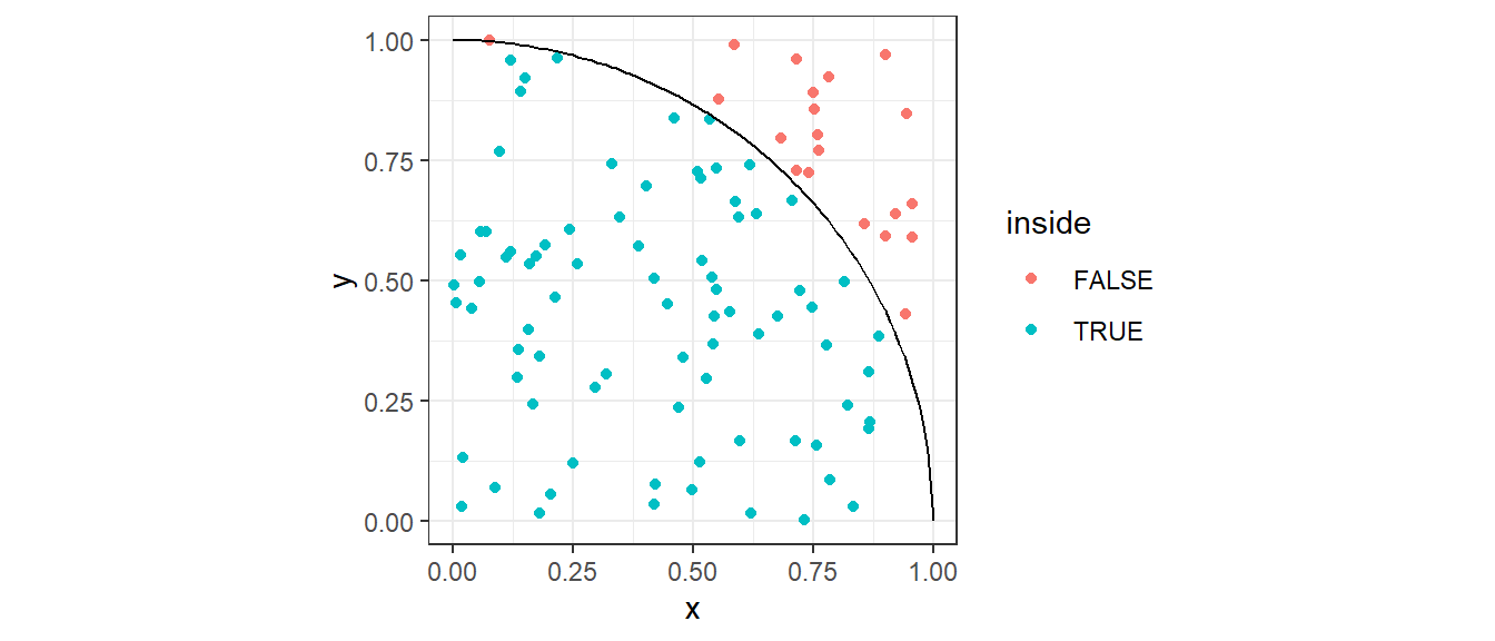
Then the final (estimated) value \(\hat{\pi}\) is 4 times the estimated area of the quarter circle.
The following algorithm can be used to approximate \(\pi\).
Generate \(M\) random points \((x,y)\) where \(x\) and \(y\) are sampled uniformly from \([0,1]\).
Count how many points fall under the quarter unit circle:
\[ x^2 + y^2 \leq 1 \]
The estimated value of \(pi\) is
\[ \pi\approx 4 \times \frac{\text{# of points in the quarter circle}}{\text{total points}} \]
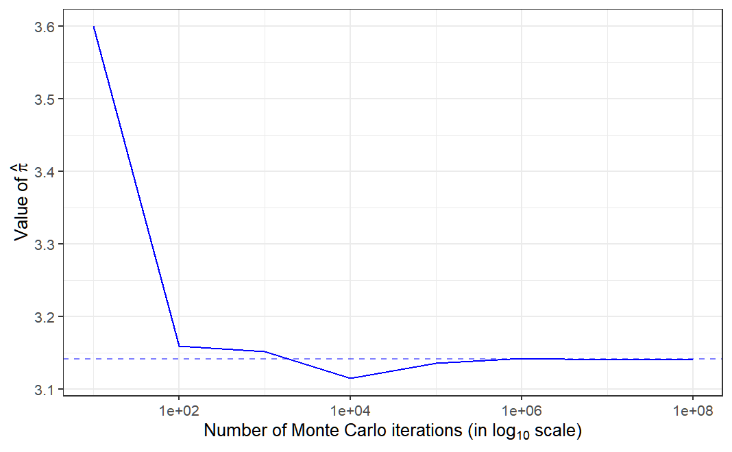
## [1] 3.13716
In fact, we can observe that as the number of Monte Carlo iterations increase, we can obtain an estimate of \(\pi\) that is closer to its actual value.
Today, the Monte Carlo method refers to any simulation that involves the use of random numbers.
9.2 Monte Carlo Probabilities
We can obtain probabilities using Monte Carlo Simulation, based on the concept of a posteriori approach of assigning probabilities.
Suppose you want to obtain the probability \(P(X\leq x)\).
The general idea for obtaining a posteriori probabilities using Monte Carlo simulation is as follows:
Generate \(M\) samples from the population \(F\).
The empirical CDF is given by
\[ \hat{F}_M(x) = \frac{1}{M}\sum_{m=1}^MI(x_m\leq x) \approx P(X\leq x) \] where \(I(.)\) is the indicator function.
Theorem 9.1 (Glivenko-Cantelli Theorem) \[ \text{As } M \rightarrow\infty, \quad\underset{x\in \mathbb{R}}{\sup}|\hat{F}_M(x)-F(x)| \rightarrow 0 \text{ almost surely} \]
Example: Exponential
Suppose \(X \sim Exp(\lambda = 1/2)\). We know that \(P(X\leq 1) = 1 - \exp(-\frac{1}{2}\cdot 1)\approx 0.39\)
If we sample large amount of times from \(Exp(1/2)\), we know that around \(39\%\) of the generated data will be less than or equal to 1.
## [1] 0.39To visualize, the following are the pdf of \(Exp(1/2)\) and the histogram of the generated dataset.
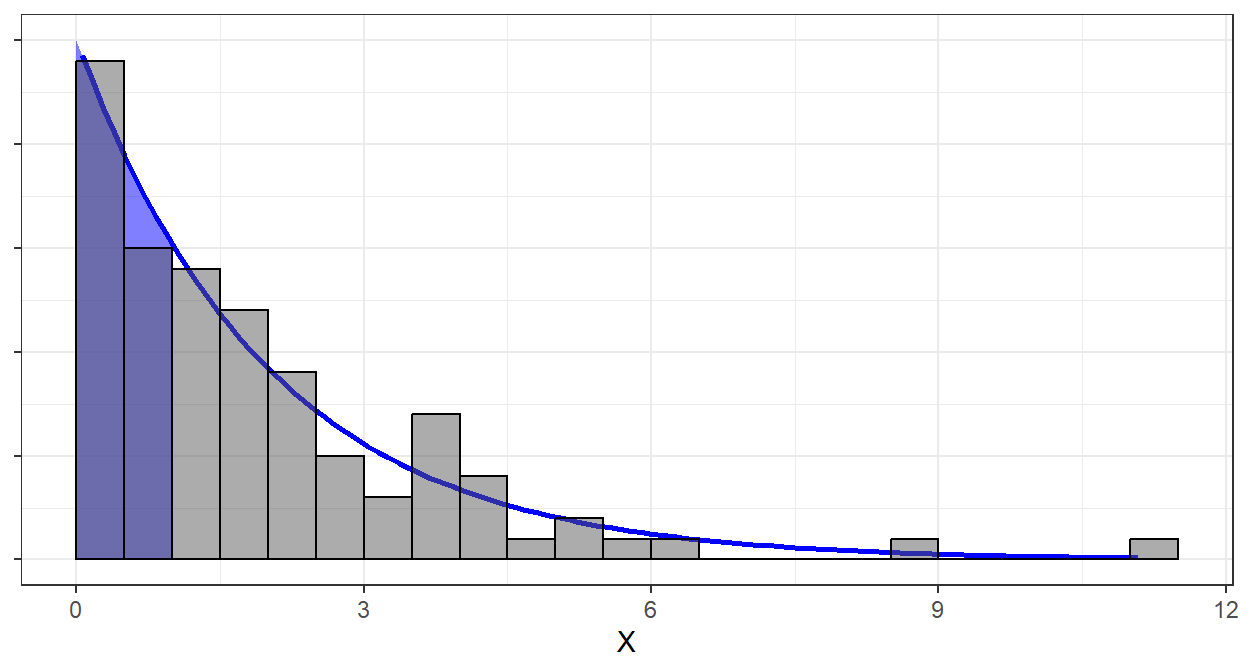
The two first bars represent \(39\%\) of the generated dataset. Likewise, the blue shaded area represents \(39\%\) of the total area under the curve and \(x\leq1\).
Alternatively, we can also plot the theoretical and empirical cdf to check if they really look the same.

By Glivenko-Cantelli Theorem, at higher \(n\), the graph of the ecdf should be smoother and will align more to the cdf.
Exercises
Let \(X\) be a random variable that is uniformly distributed over \([−1, 1]\) and \(Y\) is a random variable from \(N(1, 1)\) that is independent of \(X\). Using Monte Carlo Simulation with \(M=1000\) and seed number = 142, what is the probability that \(X + Y > 1.5\)?
Write a function to compute a Monte Carlo estimate of the \(Beta(3, 3)\) cdf. Use
rbetato generate the data. Use the function to estimate \(F(x)\) for \(x = 0.1, 0.2, . . ., 0.9\). Compare the estimates with the values returned by thepbetafunction in R.Suppose that \(X\) and \(Y\) are independent random variables variables, \(X ∼ Beta(a, b)\) and \(Y ∼ Beta(r, s)\).
Obtain a Monte Carlo estimate of \(P(X<Y)\) for \((a,b) = (10,20)\) and \((r,s)=(5,5)\)
Compare it with the derived value:
\[ P(X < Y) = \sum_{k = \max(r-b,0)}^{r-1} \frac{{{r+s-1} \choose k} {{a+b-1} \choose {a + r -1-k}} }{{a+b+r+s-2} \choose {a + r -1}} \]
You may use the function
choose(n,k)to calculate \(\binom{n}{k}\)
9.3 Law of Large Numbers
The Law of Large Numbers (LLN) is one of the pillars that makes simulations meaningful — it’s the mathematical guarantee that what we see in a simulation approximates the real quantity we’re trying to estimate if we run enough trials.
Theorem 9.2 (Weak Law of Large Numbers)
Let \(X_1,...,X_n\) be an iid random sample with \(E(X_i)=\mu\) and \(Var(X_i) = \sigma^2 <\infty\). Then for every \(\varepsilon>0\):
\[ \lim_{n\rightarrow \infty}P(|\bar{X}_n-\mu|<\varepsilon) = 1 \] That is, \(\bar{X}_n\) converges in probability to \(\mu\).
Theorem 9.3 (Strong Law of Large Numbers)
Let \(X_1,...,X_n\) be an iid random sample with \(E(X_i)=\mu\) and \(Var(X_i) = \sigma^2 <\infty\). Then for every \(\varepsilon>0\):
\[ P(\lim_{n\rightarrow \infty}|\bar{X}_n-\mu|<\varepsilon) = 1 \]
That is, \(\bar{X}_n\) converges almost surely to \(\mu\)
Most methods in the Monte Carlo framework are supported by the Law of Large Numbers. If LLN does not hold, simulation results would stay erratic no matter how many trials we run.
The LLN is the reason we can trust simulation averages to reflect true probabilities, expectations, or other parameters, provided we simulate enough trials.
Example 1: the sample mean
Suppose \(X_1,...,X_n \overset{iid}{\sim} Exp (\lambda = 0.5)\).
By Law of Large Numbers, \(\frac{1}{n}\sum_{i=1}^nX_i\overset{a.s}{\longrightarrow} 2\).
## [1] 2.326253We can see here that as \(n\) approaches a very large number, \(\bar{X}_n\) gets closer to \(2\).
Example 2: Consistency of \(S^2\)
Suppose we have a sequence \(X_1,X_2,...\) of iid random variables with \(\mathbb{E}(X_i)=\mu\) and \(Var(X_i)=\sigma^2 <\infty\). Define the sample standard deviation:
\[ S^2_n=\frac{1}{n}\sum_{i=1}^n(X_i-\bar{X})^2 \]
By Chebyshev’s Inequality, we have
\[ P(|S_n^2-\sigma^2|\geq \varepsilon) \leq \frac{E(S^2_n-\sigma^2)^2}{\varepsilon^2} = \frac{Var(S_n^2)}{\varepsilon} \] Thus, a sufficient condition that \(S_n^2\) converges in probability to \(\sigma^2\) is that \(\underset{n\rightarrow\infty}{\lim}Var(S_n^2)=0\).
Therefore,
\[ \lim_{n\rightarrow\infty}P(|S_n^2-\sigma^2|\geq \varepsilon) = 0 \]
\(S_n^2\) converges in probability to \(\sigma^2\).
## Warning: Removed 1 row containing missing values or values outside the scale range (`geom_line()`).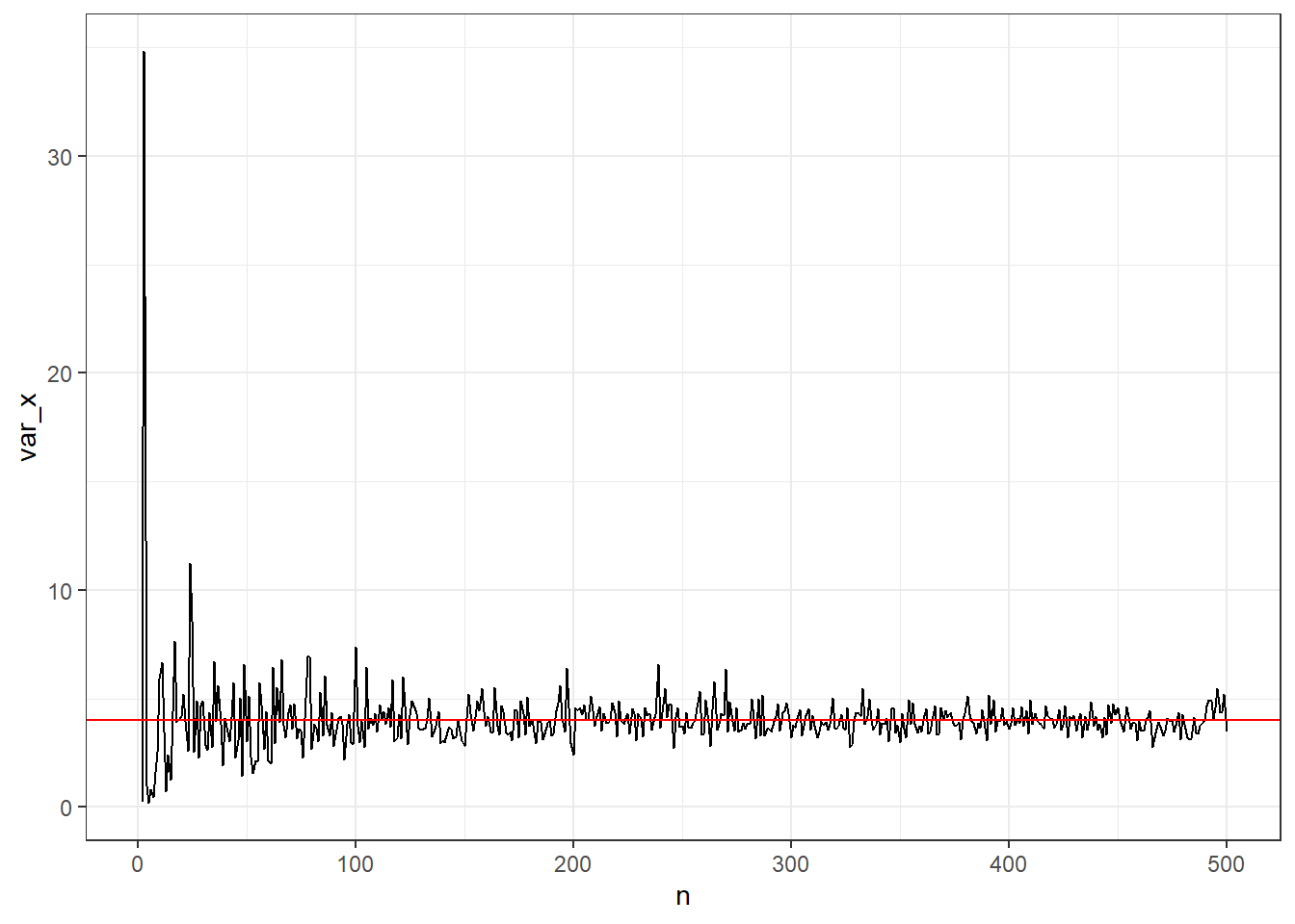
Extensions to any function
By the weak law of large numbers, for a random sample \(X_1,...\) each with same mean \(E(X)\), then
\[ \frac{1}{n}\sum_{i=1}^nX_i\overset{p}{\rightarrow}E(X) \]
A natural extension of the weak law of large numbers relates to function of random variables
\[ \frac{1}{n}\sum_{i=1}^n f(X_i)\overset{p}{\longrightarrow} \mathbb{E}[f(X)] \]
For example, suppose \(X\sim N(0,1)\). We know that \(X^2 \sim \chi^2_{(df=1)}\) and \(E(X^2)=1\). To demonstrate for a sequence of realizations \(x_1,x_2,..x_n\) of \(X\), we have the following:
## [1] 0.9451379The next section shows the application of LLN in numerical computations.
Application of law of large numbers in sampling distributions and inference will be discussed more in Chapter 10.
9.4 Monte Carlo Integration
Suppose we want to evaluate a definite integral:
\[ \int_a^b f(x)dx \]
where \(f\) is some function. For most functions, there is no closed-form expression for such definite integrals.
Numerical analysis provides various means of approximating definite integrals, starting with Euler’s method for one-dimensional integrals:
\[ \int_a^bf(x)dx\approx\sum_{i=1}^{\lfloor(b-a)/h \rfloor} hf\left(a+ih\right) \]
However, using this method is very slow, especially for high-dimensional computing. One has to evaluate the function \(f\) many times. As an alternative, physicists has to rely on some random approximation scheme, or the Monte Carlo Method.
Recall that the expected value of \(f(X)\) with respect to a distribution with probability density \(p\) with a support \(D\) is
\[ \mathbb{E}_p[f(X)]=\int_D f(x)p(x)dx \]
Based on law of large of numbers, for IID random variables \(X_1,..,X_n\) with distribution function \(p\), the sample mean of \(f(X_i)\) converges (almost surely and in probability) to the expected value of \(f(X)\):
\[ \frac{1}{n}\sum_{i=1}^nf(X_i)\rightarrow\mathbb{E}[f(X)]=\int_{D} f(x)p(x)dx \]
Example 1: Bounded Integral
The most basic Monte Carlo method for evaluating the bounded definite integral \(\int_a^b f(x)dx\) is to set \(p\) as the pdf of a Uniform random variable.
Draw the random variable \(X\) uniformly over the domain \([a,b]\), which has a pdf \(\frac{1}{b-a}\)
\[ \begin{align} \int_a^b f(x)dx &=(b-a)\int_a^b f(x) \frac{1}{b-a} dx \\ &=(b-a)\mathbb{E}[f(X)] \end{align} \]
and by law of large numbers,
\[ \frac{b-a}{n}\sum_{i=1}^n f(X_i)\rightarrow\int_a^b f(x)dx \]
To demonstrate, let us perform integration on \(f(x)=\sin(x)\) over \([0,\pi]\). The exact solution is
\[ \int_0^\pi\sin(x)dx=2 \]
Using Monte Carlo integration, we can approximate it with these steps:
Generate \(n=10000\) values from \(Uniform(0,\pi)\)
Evaluate \(f(x)=\sin(x)\) at these points
Get the average and multiply by the measure of the domain, which is \(\pi-0\).
Example 2: Unbounded Integral
Sampling from the uniform distribution is useless for an integral like
\[ \int_0^\infty x^2e^{-x^2}dx \]
The trick is to introduce a pdf with the same support as the integral limits. In general,
\[ \int_D f(x)dx=\int_D \frac{f(x)}{p(x)}p(x)dx = \mathbb{E}_p\left[\frac{f(X)}{p(X)}\right] \]
And now, if \(X_i\) is generated from \(p\),
\[ \frac{1}{n}\sum_{i=1}^n\frac{f(X_i)}{p(X_i)} \rightarrow \mathbb{E}_p\left[\frac{f(X)}{p(X)}\right] = \int_D f(x)dx \]
Solution for Example 2
Suppose we have the following integral
\[ \int_0^\infty x^2e^{-x^2}dx \]
The exact solution for this is \(\sqrt{\pi}/4\)
The Exponential distribution has bounds \([0,\infty)\), and has pdf \(\lambda e^{-\lambda x}\).
We can sample from \(Exp(\lambda = 1)\) to solve the above integral.
\[ \begin{align} \int_0^\infty x^2e^{-x^2}dx &= \int_0^\infty \frac{e^{-x}}{e^{-x}}x^2e^{-x^2}dx\\ &= \int_0^\infty \frac{x^2e^{-x^2}}{e^{-x}}e^{-x}dx\\ &= \int_0^\infty x^2e^{-x^2+x}e^{-x}dx \\ &= \mathbb{E}(X^2\exp(-X^2+X)) \end{align} \] where \(X\sim Exp(1)\)
## [1] 0.4438553## [1] 0.4431135
References
Casella, G., & Berger, R. L. (2002). Statistical inference. Brooks/Cole.
Rizzo, M. L. (2007). Statistical Computing with R. In Chapman and Hall/CRC eBooks. https://doi.org/10.1201/9781420010718
Shazili, C. (2013). Lecture Notes on Monte Carlo and Markov Chains. Carnegie Mellon University, Department of Statistics and Data Science.
https://www.stat.cmu.edu/~cshalizi/statcomp/13/lectures/15/lecture-notes-markov.pdf