1.1 Rules of Programming
From top to bottom
Instructions are executed sequentially.
In most (if not all) programming languages, instructions are executed sequentially, from top to bottom. For example, if we have the following instructions, line 1 will be executed first, followed by line 2.
## [1] 6
## [1] 3
The first line will be executed first before the second line.
The following is another example where there are two assignment statements on the object x.
Our computers do not get confused what we mean by x in line 3, because all instructions are executed sequentially.
Expressions first
Expressions are evaluated before instructions are executed.
An expression is a combination of operators, constants and variables. An expression may consist of one or more operands, and zero or more operators to produce a value.
Below is a sample code.
## [1] 60In the first line, 2 + 4 is an expression. This will be evaluated first, before the whole instruction (which is the assignment) will be executed.
In the second line, x - 1 is evaluated before storing the value to y.
In the last line, 2*x*y is evaluated before the print instruction is executed.
Hierarchy of Environments
Names are evaluated using the hierarchy of environments
Remember this operator: <-? This is called the assignment operator.
What it does is create a bind between the value (or more generally the object) on the right of it to the name of the left.
<NAME> <- <OBJECT>Hence, the name is associated with the object (which exists virtually in our computer’s memory).
Consequently, an object can be associated with many different names.
Here, the object 2 is only a single entity, i.e., we are not creating multiple copies of the entity 2.
Rather, we are associating 2 with different names—x, y, and z. In short, 2 can be called using x, y, and z.
But note that the assignment operator is unidirectional—it doesn’t go both ways.
It means that, while an object can be associated with many different names, a name can only be associated with a single object.
That’s why, in the lines of code above, the second line rebinds the name x to the new value 3, and when x is called after running the lines of code, 3 will be returned by the computer and not 2.
But, if names have to be unique, does this mean you cannot repeat a name when you want to refer to different objects?
- While an object can be associated with many different names, a name can only be associated with a single object in a particular environment.
So what is an environment?
- An environment is a collection of name-object bindings (which are located in a frame) + the environment’s parent environment.
Consider the following bindings below done in the global environment (our default working environment).
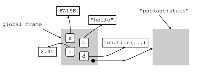
What is this telling us?
the four name-object bindings we made above are found in the global frame (i.e., the frame of the global environment), and
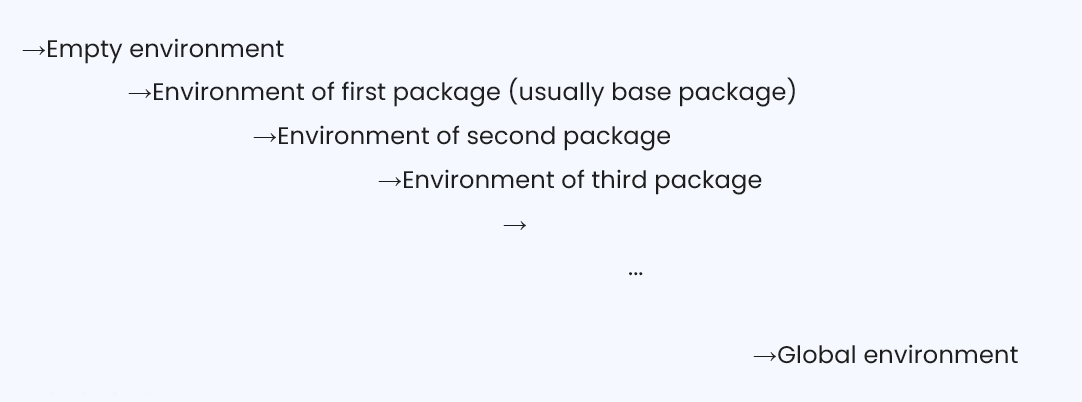
global frame + the global environment’s parent environment (which in this case is package:stats) are what make up the global environment.
What do we mean by “a name can only be associated with a single object in a particular environment”?
Well, it means that, in a particular environment—say, the global environment—the name
arefers toFALSEonly,bto"hello"only, and so on.But, in a different environment, these names can be bound to different values or objects.
Why is this relevant?
First, we can reuse names without our computers getting confused. Depending on the context—the environment—in which the computer is operating on, a particular name will refer to a particular object relevant to that context.
Second, our names don’t have to be convoluted. We can keep them simple like
counter,n,i, etc., and use them for a particular context we are working on.Third, it gives us the ability to simplify complex tasks.
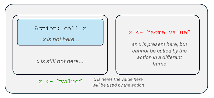
If we call a name in a particular environment, our computer will:
Look for a binding to that name in the frame of the environment.
- If a binding was found, our computer will return the object associated with that name.
- If not, our computer will go to the parent environment of the particular environment.
- In the parent environment of the particular environment, our computer will look for a binding to that name.
- If a binding was found, our computer will return the object associated with that name.
- If not, our computer will go to the grandparent environment of the particular environment. And so on….
- In the parent environment of the particular environment, our computer will look for a binding to that name.
Why are environments important?
They give context to the names that we are calling in our computer, so that the name we can use to bind to our objects will not necessarily be unique.
Hierarchy
More about this in Section 1.2.1 .
Functions as abstractions
first, it interrupts the sequential execution of instructions in the parent environment,
then proceeds with the execution of the instructions defined inside the function in a new environment.
What is “abstraction” in programming?
In object oriented programming, abstraction is a fundamental concept that simplifies complex systems by focusing on essential characteristics while concealing unnecessary details.
It is a way of hiding complicated details from the end user.
There is a term called “don’t repeat yourself” or “DRY” in programming, which suggests that it is a good programming practice to NOT use a block of code, or information, repeatedly.
What we want is to be able to “abstract” this information, i.e., define an object we can call multiple times without having to reveal ALL unnecessary information.
Creating “functions” helps us in abstraction.
Function in R
Note that a function is defined in R with the following syntax:
<NAME OF FUNCTION> <- function(<ARGUMENT 1>, <ARGUMENT 2>, ...){
  <FIRST INSTRUCTION OF THE FUNCTION>
  <SECOND INSTRUCTION OF THE FUNCTION>
  ...
}
This means that the class of <NAME OF FUNCTION> is a function, regardless of the instructions inside it.
More details about this in Section 1.2 .
Questions
What is the value of
xin the global environment after this sequence of codes?What will be bound to
a,b, andxin the global environment after the function was called?
All about context
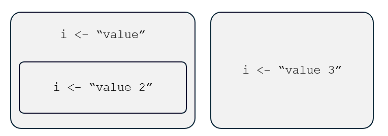
Each time a function is called, bindings are created in a separate environment.
| Name | Global Environment | New Environment
|
New Environment
|
|---|---|---|---|
x |
3 |
2+5=7 |
3+5=8 |
a |
5 |
5 |
5 |
b |
2 |
x=3 |
|
func |
<definition> |
Returns as a form of control
A return is a statement that interrupts the execution of a function call.
There are two ways we can instruct our computers to go back to the environment where the function was called.
We just wait for the computers to finish all instructions defined inside the function that was called.
We call the
returnstatement.- When the computer encounters this statement, it will stop executing the remaining instructions inside a function, then return to the environment where the function was called—together with whatever is included inside the parentheses of the statement
- (i.e.,
return(<AN OBJECT TO BE RETURNED>).
## [1] 7
return refers to an instruction for the computer to stop doing whatever it is doing inside the function, then return to wherever it is called.
What does this mean?
Recall that during a function call, our computers shift from the parent environment (where the function was defined) to the new environment (which is created when the function was called).
In the new environment, our computers will do whatever instructions were defined inside the function which was called.
return will not proceed with any commands after it, and will return to the parent environment.
## [1] 7More powerful forms of control
Control structures alter the sequential execution of instructions.
The first rule of programming we learned is the instructions are executed, from top to bottom. This doesn’t give us much power to do complex tasks. Previously, we also learned that we could use the return statement to alter that sequential execution.
We take this a step further with control structures.
If we want to skip some steps based on some conditions, we use selection control structures. These are the if-else-then statements that are very common in all programming languages.
On the other hand, if we want to execute commands repeatedly, we use repetition control stuctures. These are the for loop, while loop, until loop, and other structures that allows the computer to continuously execute commands while conditions are satisfied.
More of this in Section @(control)
Data as abstractions
Data structures allow us to represent individual objects as a single entity.
Suppose we have the following dataset.
| y | assignedSex | age |
|---|---|---|
| 3 | F | 30 |
| 2 | M | 28 |
| 7 | F | 35 |
Each cell value can be assigned to some object.
y1 <- 3
y2 <- 2
y3 <- 7
assignedSex1 <- "F"
assignedSex2 <- "M"
assignedSex3 <- "F"
age1 <- 30
age2 <- 28
age3 <- 35
Data structures allow us to make sense of different values that have relationships with each other.
##   y assignedSex age
## 1 3           F  30
## 2 2           M  28
## 3 7           F  35
Types of Data Structures
Atomic vector
the most fundamental data structure in R. It is a single dimension structure which can only contain a single type of data (e.g., only numbers or only character strings). By default, everything we create in R are atomic vectors.
my_log <- c(TRUE, FALSE, T, F, NA) my_int <- c(1L, 2L, 3L, 4L, NA) my_dbl <- c(1.25, 1.50, 1.75, 2.00, NA) my_chr <- c("a", "b", "c", "d", NA)## [1] TRUE FALSE TRUE FALSE NA ## [1] 1 2 3 4 NA ## [1] 1.25 1.50 1.75 2.00 NA ## [1] "a" "b" "c" "d" NAMatrix
An extension of vector data in two dimensions
##      [,1] [,2] [,3]
## [1,]    1    4    7
## [2,]    2    5    8
## [3,]    3    6    9
Array
an extension of the vector data structure to n-dimensions.
# example: 3 dimensional array
# 3 rows, 4 columns, 2 layers
arr <- array(1:24, dim = c(3, 4, 2))
print(arr)
## , , 1 ## ## [,1] [,2] [,3] [,4] ## [1,] 1 4 7 10 ## [2,] 2 5 8 11 ## [3,] 3 6 9 12 ## ## , , 2 ## ## [,1] [,2] [,3] [,4] ## [1,] 13 16 19 22 ## [2,] 14 17 20 23 ## [3,] 15 18 21 24List
like vectors but they allow different kinds of object per element
## [[1]]
## [1] "hello world"
##
## [[2]]
## [1] 1.25 1.50 1.75 2.00   NA
##
## [[3]]
##      [,1] [,2] [,3]
## [1,]    1    4    7
## [2,]    2    5    8
## [3,]    3    6    9
##
## [[4]]
## , , 1
##
##      [,1] [,2] [,3] [,4]
## [1,]    1    4    7   10
## [2,]    2    5    8   11
## [3,]    3    6    9   12
##
## , , 2
##
##      [,1] [,2] [,3] [,4]
## [1,]   13   16   19   22
## [2,]   14   17   20   23
## [3,]   15   18   21   24
Data frame
a special type of list, containing atomic vectors with the same length.
names  <- c("Aris", "Bertio", "Condrado", "Dionisia", "Encinas")
age    <- c(22L, 20L, 21L, 18L, 19L)
grade  <- c(3.00, 2.25, 2.50, 1.00, 1.50)
class_data <- data.frame(names, age, grade)
The following dataframe has 3 columns (variables) and 5 rows (observations).
names<chr>age<int>grade<dbl>Aris 22 3.00 Bertio 20 2.25 Condrado 21 2.50 Dionisia 18 1.00 Encinas 19 1.50
In R, we are lucky to have several—including data frames, which are really suitable when working with data sets. The base data structures of R can be categorized by the number of their dimensions, and whether they’re homogeneous or heterogeneous.
| Data Structure | Dimensions? | Heterogeneous? |
|---|---|---|
| Atomic vector | 1 | No |
| List | 1 | Yes |
| Matrix | 2 | No |
| Data frame | 2 | Yes |
| Array | n | No |
The term data structure is actually a misnomer, because they can hold, not only data, but also other objects—like functions, or other collections of objects.
simple_model <- lm(y ~ x, data=data.frame(y = c(1, 3, 5, 3), x = c(1, 2, 3, 4)))
summary(simple_model)
##
## Call:
## lm(formula = y ~ x, data = data.frame(y = c(1, 3, 5, 3), x = c(1,
## 2, 3, 4)))
##
## Residuals:
## 1 2 3 4
## -0.8 0.4 1.6 -1.2
##
## Coefficients:
## Estimate Std. Error t value Pr(>|t|)
## (Intercept) 1.0000 1.8974 0.527 0.651
## x 0.8000 0.6928 1.155 0.368
##
## Residual standard error: 1.549 on 2 degrees of freedom
## Multiple R-squared: 0.4, Adjusted R-squared: 0.1
## F-statistic: 1.333 on 1 and 2 DF, p-value: 0.3675Usually, when complex objects are represented on our computers, e.g., regression models, a combination of different kinds of objects—not only data or values—are combined.
Exercise 1.1
In your devices, open R Studio and create an R project. This shall be your working environment.
Explore how to work with R Markdown.
Visit this link to know more about text formatting and other capabilities of R Markdown:
Note that for our machine problems, I will be requiring you to use R Markdown for easier documentation. Results must be knitted to PDF.