2.2 Measuring Program Complexity

When developing algorithms, understanding their efficiency is crucial for writing optimized code.

Performance and complexity are closely related, but they are different.

Performance: how much time/memory/disk/… is actually used when a program is run. This depends on the machine, compiler, etc. as well as the code.
Complexity: how do the resource requirements of a program or algorithm scale, i.e., what happens as the size of the problem being solved gets larger?

In other words, complexity affects performance, but not the other way around.

The efficiency of an algorithm is often analyzed using Big-O notation, which describes how the runtime or space requirements grow as the input size increases.

This chapter explores programming complexity, common complexity classes, and practical examples using R.

2.2.1 Understanding Big-O

When we are trying to find the complexity of the function/procedure/algorithm/program, we are NOT interested in the exact number of operations that are being performed. Instead, we are interested in the relation of the number of operations to the problem size.

Typically, we are usually interested in the worst case: what is the maximum number of operations that might be performed for a given problem size.

Definition 2.3 Big-O notation is a mathematical representation of an algorithm’s growth rate. It helps predict performance as input size ( $n$ ) increases. The notation describes the upper bound of an algorithm’s running time.

Formally, it is defined as the following:

Let $f$ be a real or complex valued function and $g$ a real valued function. Let both funtions be defined on some unbounded subset of the positive real numbers, and $g(n)$ be strictly positive for all large enough values of $n$ . Then

$f(n) \rightarrow O(g(n)) \quad \text{as} \quad n \rightarrow\infty$

if the absolute value of $f(n)$ is at most a positive constant multiple of $g(x)$ for all sufficiently large values of $x$ .

That is, $f(n)= O(g(n))$ if there exists a positive real number $c$ and a real number $k$ such that

$|f(n)| \leq c|g(n)| \quad \forall \quad n \geq k$

The notation is read, “f of n is big oh of g of n”.
Saying some equation $f(n) = O(g(n))$ means it is less than some constant multiple of $g(n)$ .This may also be interpreted as “A function $f(n)$ belongs to the set $O(g(n))$ if it less than or equal to $c\times g(n)$ ”
Informally, O-notation characterizes an upper bound on the asymptotic behavior of a function $f()$ . In other words, it says that a function grows no faster than a certain rate, based on the highest-order term.
In Cormen et.al (2022), the absolute value bars are discarded, since only positive functions are considered.
In more simple terms, this measures the maximum complexity of an algorithm
For a given input of size $n$ , how much more complex will the algorithm be?
Basically, it tells you how fast a function grows or declines. Landau’s symbol comes from the name of the German number theoretician Edmund Landau who invented the notation. The letter $O$ is used because the rate of growth of a function is also called its order.

There are two types of complexities that we can use the $O$ -notation: time complexity and space complexity.

We will focus on the time complexity, since this is just an introduction. We won’t focus much on the theory, as we rarely encounter this as statisticians.

2.2.2 Determining Time Complexities

The time required by a function/procedure is proportional to the number of “basic operations” that it performs. Here are some examples of basic operations:

one arithmetic operation (e.g., a + b, x * y);
one assignment (e.g. x <- 0);
one test (e.g., x == 0);
one read (of a primitive type: integer, float, character, boolean); and
one write (of a primitive type: integer, float, character, boolean)

But again, we are not interested in the exact number of basic operations that are being performed. Instead, we are interested in the relation of the number of operations to the problem size.

For example, in the algorithm below, the number of elements of x determines the the number of operations to be performed.

x <- c(1, 2, 3, 4, 5)
mean <- function(x){
  i <- 1
  sum <- 0
  while(i <= length(x)){
    sum <- sum + x[i]
    i <- i + 1
  }
  return(sum/length(x))
}
mean(x)

The number of elements here is the problem size or input size. If you increase the number of elements, the number of operations will also increase linearly.

Note that the big-O expressions do not have constants or low-order terms.

For example:

$O(N+2)\rightarrow O(N)\\ O(N^2 + N) \rightarrow O(N^2)$

This is because, when $N$ gets large enough, constants and low-order terms don’t matter (a constant-time algorithm will be faster than a linear-time algorithm, which will be faster than a quadratic-time algorithm).

The following are some basic properties of the Big-O notation:

Sequence of Statements
```
statement 1
statement 2
...
statement k
```
The total time is found by adding the times for all statements:

$\text{total time} = \text{time}(\text{statement 1}) + \text{time}(\text{statement 2}) + \cdots + \text{time}(\text{statement n} )$ If each statement is “simple” (only involves basic operations) then the time for each statement is constant and the total time is also constant: $O(1)$ .

Even if an algorithm executes a fixed number of steps (e.g., 2, 3, or 10 operations), it is still considered $O(1)$ because the execution time does not grow with $n$ .
If-then-else
```
if(cond){
    block 1 (sequence of statements)
}else{
    block 2 (sequence of statements)
}
```
Here, either block 1 will execute, or block 2 will execute. The worst-case time is the slower of the two possibilities:

$\max\{\text{time}(\text{block 1}), \text{time}(\text{block 2})\}$

Again, the Big-O characterizes the maximum complexity of the algrotihm. If block 1 takes $O(1)$ and block 2 takes $O(N)$ , the if-then-else statement will be $O(N)$ .
Loops
```
for(i in 1:N){
    sequence of statements
}
```
The loop executes $N$ times, so the sequence of statements also executes $N$ times. If we assume the statements are $O(1)$ , the total time for the for loop is $N\times O(1)$ , which is $O(N)$ overall.
Nested Loops
```
for(i in 1:N){
    for(j i in 1:M){
    sequence of statements
    }
}
```
The outer loop executes $N$ times. Every time the outer loop executes, the inner loop executes $M$ times. As a result, the statements in the inner loop execute a total of $N\times M$ times. Thus, the complexity is $O(N\times M)$ .

A common case is if the inner loop also executes $N$ times, then the complexity is $O(N^2)$ .
Statements with function calls

When a statement involves a function/procedure call, the complexity of the statement includes the complexity of the function/procedure.

Assume that you know that function/procedure $f$ takes constant time, and that function/procedure $g$ takes time proportional to (linear in) the value of its parameter $k$ . That is,
- $f(k)$ has $O(1)$
- $g(k)$ has $O(k)$
When a loop is involved, the same rule applies. For example:
```
for (j in 1:N){
    g(j)
}
```
has complexity $O(N^2)$

Explanation

The total complexity is given by

$O(1) + O(2) + \cdots + O(N)$

Which forms

$\begin{align} O(1 + 2 + \cdots + N) &= O\left(\sum_i^N i \right) \\ &= O\left(\frac{N(N+1)}{2}\right)\\ &= O\left(\frac{N^2}{2}+\frac{N}{2}\right) \end{align}$

In Big-O notation, we drop constant factors and retain the highest order. This simplifies to:

$O(N^2)$

This quadratic complexity arises because later iterations take increasingly more time to execute, and their cumulative effect results in a growth rate proportional to $N^2$

2.2.3 Common Time Complexity Cases

There are many complexity cases. In the following, we only show cases for algorithms with only one dimension of input size parameter $n$ .

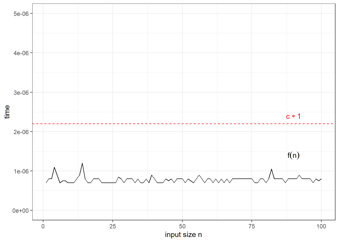
$O(1)$ : Constant Time

Execution time is independent of input size.

Example: Indexing

Fetching an element from a vector takes constant time, regardless of its size.

get_element <- function(arr, index) {
        return(arr[index])
}

# Example usage:
my_array <- c(10, 20, 30, 40, 50)
get_element(my_array, 3)  # Returns 30

## [1] 30

Accessing an element in an array by index happens in a single step, regardless of whether the array has 10 or 10 million elements. This is why we say the order is 1 — the time taken is independent of $n$ .

Visualization

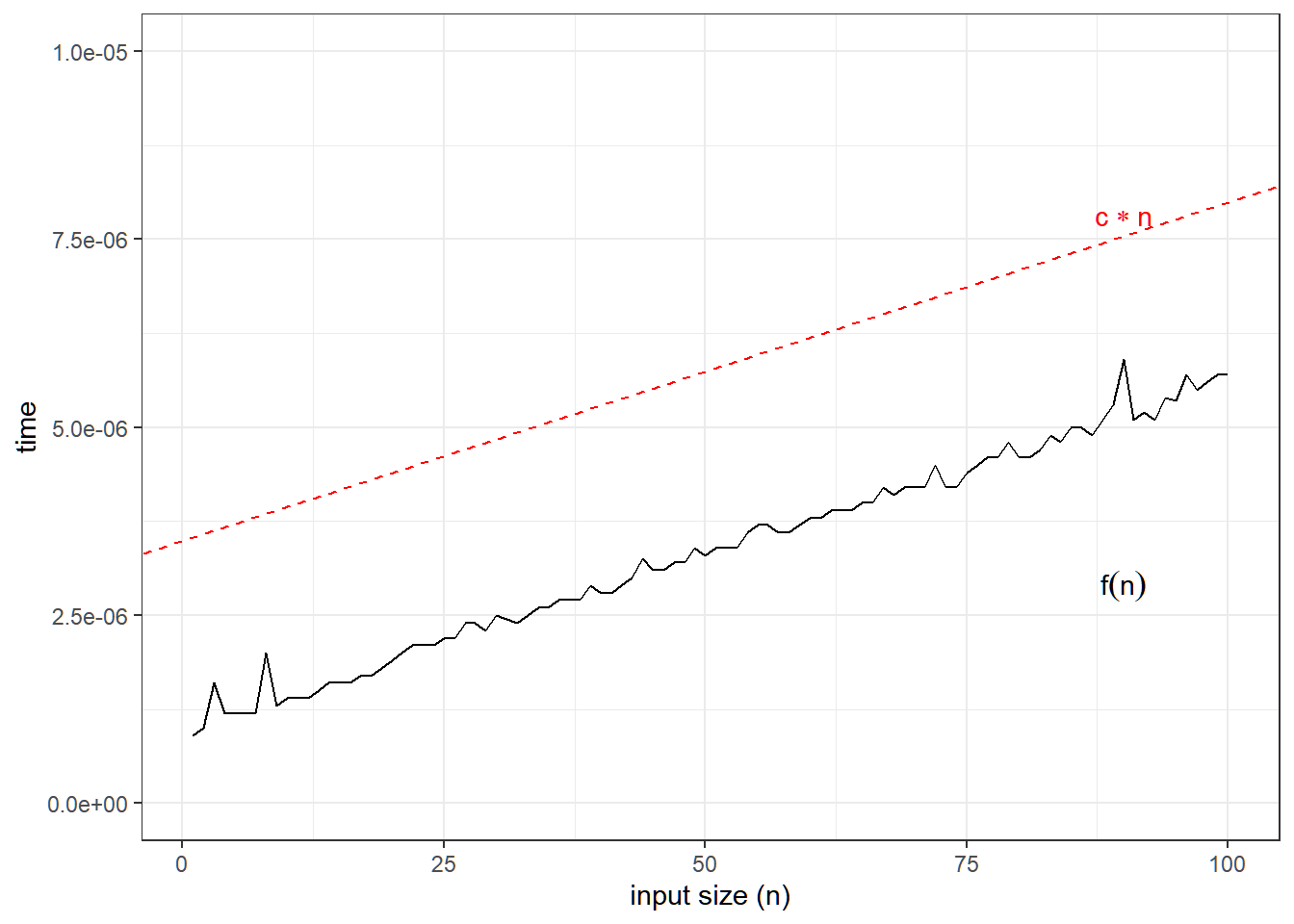
$O(n)$ : Linear Time

Execution time increases linearly with input size.

Example: Linear Search

A linear search algorithm checks each element until it finds a match. Here, the input size is the number of elements.

linear_search <- function(arr, target) {
    for (i in seq_along(arr)) {
        if (arr[i] == target) {
            return(i)
        }
    }
    return(-1)
}

# Example usage:
linear_search(my_array, 30)  # Returns index of 30

## [1] 3

The basic operation here is the test arr[i] == target. It takes exactly one unit of time to loop each over element, and the worst case scenario here is if the target is at the end of the array. In other words, upper bound for the number of tests arr[i] == target is n.

Visualization

In linear search, fastest case scenario is if the element to search is the first element, and the slowest case scenario is if the element to search is the last element.

Let’s assume that we are searching an element that is unfortunately the last, yielding to the slowest program run time.

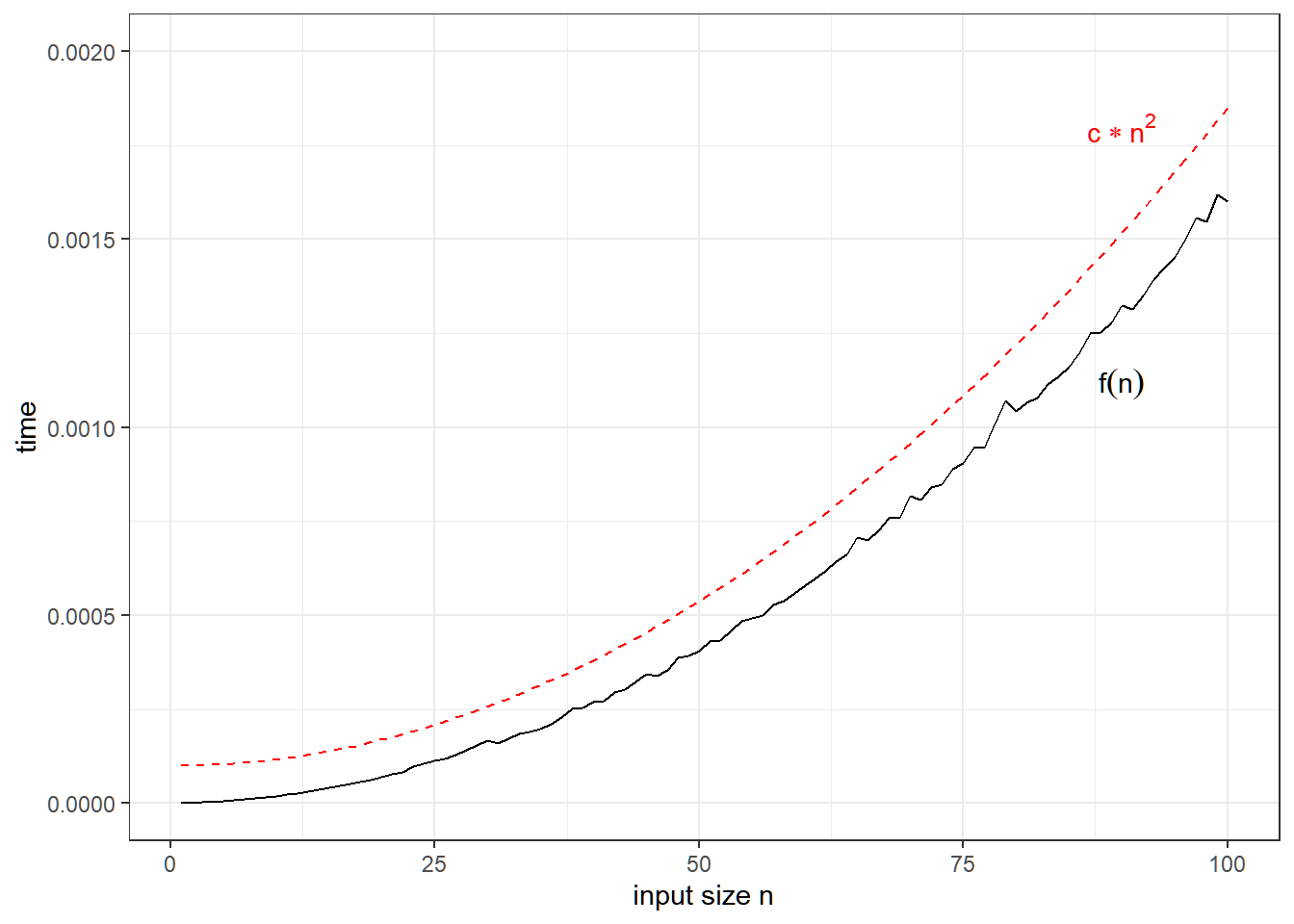
$O(n^2)$ : Quadratic Time

Execution time is proportional to the square of the input.

Example: Nested Loop

A nested loop leads to quadratic complexity

nested_loop <- function(n) {
    for (i in 1:n) {
        for (j in 1:n) {
            print(paste("i:", i, "j:", j))
        }
    }
}

# Example usage:
nested_loop(3)  # Runs 3x3 = 9 times

## [1] "i: 1 j: 1"
## [1] "i: 1 j: 2"
## [1] "i: 1 j: 3"
## [1] "i: 2 j: 1"
## [1] "i: 2 j: 2"
## [1] "i: 2 j: 3"
## [1] "i: 3 j: 1"
## [1] "i: 3 j: 2"
## [1] "i: 3 j: 3"

The basic operation is print(paste("i:", i, "j:", j)), which will run $n^2$ times.

Visualization

$O(\log n)$ : Logarithmic Time

Execution time grows logarithmically with input. This scales much better for larger number of inputs.

Example: Binary Search

Binary search works by dividing the search space in half, achieving logarithmic complexity:

binary_search <- function(arr, target) {
  left <- 1
  right <- length(arr)
  while (left <= right) {
    mid <- floor((left + right) / 2)
    if (arr[mid] == target) {
        return(mid)
    } else if (arr[mid] < target) {
        left <- mid + 1
    } else {
        right <- mid - 1
    }
  }
  return(-1)
}

# Example usage:
my_sorted_array <- c(10, 20, 30, 40, 50)
binary_search(my_sorted_array, 30)  # Returns index of 30

## [1] 3

How Binary Search works?

Start with a sorted list.
Compare the target value with the middle element.
- If it’s the middle element, return its index.
- If it’s smaller, search in the left half.
- If it’s larger, search in the right half.
Repeat this process, halving the remaining search space each time.

Why $O(\log n)$ ?

Each step reduces the problem size by half. To solve the number of executions, we find how many times we half the input $n$ until it reaches 1.

Mathematically, this is solving for $k$ :

$\frac{n}{2^k}=1\\ k = \log_2 n$ Since Big-O ignores constants and base changes, we simplify this to $O(\log n)$ .

Visualization

In binary search, the worst case scenarios are if the element to search is either the first element or the last element.

For this visualization, we simulate for the case that the item to search is unfortunately the last element of the array.

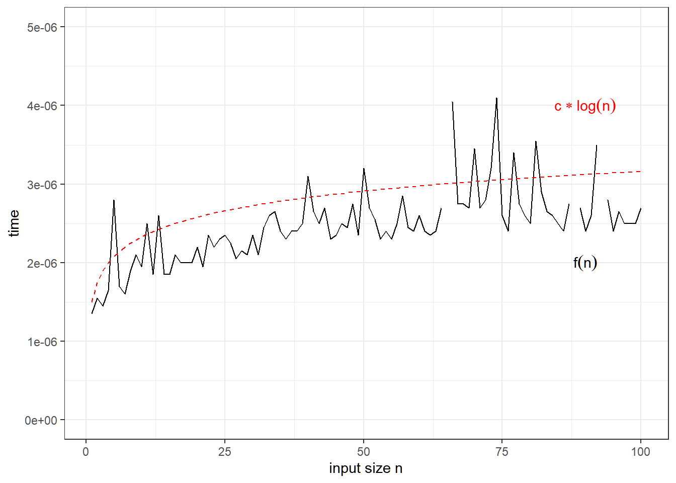
There are some program fluctuations when running the program.

$O(2^n)$ : Exponential Time

Growth doubles with each additional input element. This is common when looping for every possible combination in an array.

Example: All Possible Regressions

Recall in linear regression, one way to select the best regression model given $k$ possible predictors is through all-possible-regression approach, where you fit the $2^k-1$ possible models, then select the best based on some metrics, such as $R^2$ and Mallow’s $C_p$ .

If we assume that the number of independent variables is the input size, and fitting a linear model has complexity $O(1)$ , then the time complexity of an algorithm that shows all possible linear regression models is $O(2^k)$ .

$O(n \log n)$ : Linearithmic Time

Common in efficient sorting algorithms.

Understanding Big-O notation helps in selecting the most efficient algorithm for a given problem.

$O(1)$ and $O(\log n)$ algorithms are optimal.
$O(n^2)$ or worse should be avoided when dealing with large datasets.

R provides tools to analyze and compare algorithmic performance, helping programmers make informed decisions.

Exercises

The following are sample pseudocodes for some algorithms.

Determine the input size parameter/s and time complexity of the algorithms and implement them in R.

Counting Pairs

INPUT: numeric vector A and a number k

OUTPUT: number of pairs with sum greater than k

COUNT_PAIRS(A, k)
1.  count ← 0
2.  n ← length(A)
3.  FOR i ← 1 to n DO
4.      FOR j ← i + 1 to n DO
5.          IF A[i] + A[j] > k THEN
6.              count ← count + 1
7.          END IF
8.      NEXT j
9.  NEXT i
10. RETURN count

Insertion Sort

INPUT: a sequence of numbers $A = \langle a_1,a_2,...,a_n \rangle$

OUTPUT: a reordering $\langle a'_1,a'_2,...,a'_n \rangle$ such that $a'_1 \leq a'_2 \leq ... \leq a'_n$

INSERTION_SORT(A)
1.  FOR i from 2 to length(A) do
2.      key ← A[i]
3.      j ← i - 1
4.      WHILE j > 0 and A[j] > key do
5.          A[j + 1] ← A[j]  // Shift element to the right
6.          j ← j - 1
7.      END LOOP        
8.      A[j + 1] ← key  // Insert key at the correct position
9.  NEXT i