R
“‘I checked it very thoroughly,’ said the computer, ‘and that quite definitely is the answer. I think the problem, to be quite honest with you, is that you’ve never actually known what the question is.’”
- The Hitchhiker’s Guide to the Galaxy
We are currently in the process of editing Probability! and welcome your input. If you see any typos, potential edits or changes in this Chapter, please note them here.
##Motivation {-}
R is a very popular and incredibly useful statistical computing software. The concepts presented in this book mainly have a theoretical, non-applied tilt; however, R can still be of great use to us. Specifically, we will often leverage R to simulate complex problems that are difficult or impossible to solve analytically. These simulations will allow us to check our work and often think about our solutions in a new light. Ultimately, it’s much easier to learn about probability if you can leverage the power of a computer!
While computing in R can be very complex, we will try to keep the code in this book at a relatively introductory level. Often in computer science, the top priority is to write fast code; here, our top priority will be getting the answer right while keeping the code understandable! We will still aim for succint, efficient code, but we may bypass some of the more sophisticated, advanced programming techniques for the sake of clarity.
Further, this chapter is not meant to be a comprehensive guide to R, merely a crash-course or even refresher to allow you to be more comfortable while reading this book. For more on R, please refer to Blitzstein and Hwang (2014) or Teetor (2011).
Getting Started in R
R can be used for anything from arithmetic to sophisticated statistical analysis. If you have any experience coding in languages like C, C++, or Python, you will likely pick up R very quickly, and probably will even find it more readable than other popular languages!
It is recommended that you use RStudio (which you can download for free here). This is essentially an intuitive, user-friendly interface that supports R. It connects most of the important parts of R - the console, a script editor, the environment, plots, etc. - into one intuitive visual.
It’s probably best to start by using R as a glorified calculator to get used to working with the software. Let’s perform some basic arithmetic in R. You type these commands into the console, and then hit ‘enter’ to run them.
2 + 2## [1] 4Notice the line of code, 2 + 2, and how R returns the answer, 4, below the line of code. In your console, you only have to hit 2 + 2 and then hit enter for R to return 4. Now, let’s try some other arithmetic calculations.
2*3; 2/2; 2^2## [1] 6## [1] 1## [1] 4The semicolons used in the line of code only serve to collect all of the output together (you could also put the calculations on their own lines). Notice how, since we used the semicolon, all of the output is printed in one go (in order).
Of course, this type of arithmetic will only get us so far. We can also store values in R, or create variables with specified values, to make computations more organized. Let’s store 2 in the value x and perform the same calculations.
x = 2
x*3; x/x; x^x
## [1] 6## [1] 1## [1] 4We get the same output as the calculations above, because the value 2 is stored in x.
We can perform even more advanced arithmetic with built-in R functions. If you are not familiar with computer science, a function is essentially a tool that, when ‘called,’ performs some sort of (predefined) process. Functions take in inputs (also called arguments), perform some sort of analysis and return outputs.
In R, functions are called by name, and parentheses surround the function inputs. For example, function1(3,8) would call a function named function1 that takes 3 and 8 as its inputs. Many, many functions come predefined in R (or are available in ‘packages’ that you can download); let’s use the sqrt and exp functions here.
sqrt(1); exp(2)## [1] 1## [1] 7.389056The first function, sqrt, is (intuitively) the ‘square root function,’ which takes one input (a single number) and returns the square root of that number (notice how the parentheses surround the number). The exp, or exponential function, returns \(e^x\), where \(x\) is the input of the function. Here, we found the square root of 1 (just 1) and \(e^2\), which comes out to about 7.39.
These two examples are just the tip of the iceberg: you can use functions to analyze data sets, generate random values, and perform sophisticated statistical analysis. If you ever need help or more information about a function, you can type ?sqrt, or a question mark followed by the function name, in the console and hit return. A full help page should pop up. We will learn about writing our own functions later in this chapter.
Now let’s move from working with a one-dimensional, single-value object to analyzing a vector. If you aren’t familiar with vectors, just think of them as a list of numbers, bound together. Let’s create a vector and store it in x. We will use the c() function, which is short for ‘concatenate,’ to create the vector (essentially, it binds elements together).
Now would also be a good time to mention commenting in R. A # denotes a comment that is written in English and intended for humans; the computer will not run a line of code that starts with #. This is a good way to describe what you are doing to someone reading your code.
#create a vector
x = c(3, 1, 9)

#print x
x
## [1] 3 1 9Here, we created a vector x and printed it out; notice how it consists of three values: 3, 1 and 9. Now that we have a full vector, we can perform more complicated functions on it, like mean() and sum() (which, intuitively, return the mean and sum of their inputs).
x = c(3, 1, 9)
mean(x); sum(x)
## [1] 4.333333## [1] 13Vectors are actually quite intuitive to work with in R. For example, if you add two vectors of the same length, you get another vector of the same length, where each entry is the sum of that entry in the other two vectors (that is, R is vectorized, which is a topic for a more advanced discussion of R).
#define vectors
x = c(3, 1, 9)
y = c(2, 5, 6)

#each entry adds
x + y
## [1] 5 6 15We can also index into vectors with square brackets []. For example, we can pull out the second entry of a vector:
#create a vector
x = c(3, 1, 9)

#print 2nd element
x[2]
## [1] 1Similar to other computing languages, R also has ‘if/else’ statements, as well as ‘and/or’ logic. These can be used to alter bits of code depending on certain conditions; see the Glossary in this chapter for more. From simple calculations, functions, vectors, and basic logic, an entire world of complexity opens up.
Functions
As mentioned briefly above, functions make working in R much easier and more productive. Many functions are predefined in the base R package (i.e., sqrt and exp, per the examples above) and many more have been written in packages that are available for download; however, you often need to write your own function to address a very specific need.
If you are familiar with writing functions in other languages, the logic for writing functions in R is extremely similar. If you are not familiar, recall that functions take inputs (also called arguments) and, based on these inputs, performs some sort of analysis and return outputs. Let’s define a simple function below.
#define a function
my.first.function = function(x){

  #return the square of x
  return(x^2)
}

#call the function
my.first.function(2)
## [1] 4There are a couple of important bits of code here that we need to discuss. First, my.first.function is the name of the function that we created, and the way that we will call the function from the moment it is defined. Now consider the = function(x) part of the code chunk. This bit of code says to make my.first.function into a function, and for this function to take one argument (here it is called x). We could define a function that takes two or more arguments by writing function(x, y), etc. Then, we have two curly braces {}, inside of which we perform the function’s main task. Here, we want to ‘return’ the square of the value we entered, so we put x^2 inside of return(x). Again, the reason we use x here is because we entered x as our argument in function(x); it doesn’t actually matter what we call the argument, as long as we are consistent between the argument and the body of the function! Finally, notice how we called the function after we defined it, passing it the argument 2. As expected, the function correctly returned the value 4, which of course is just \(2^2\).
Consider defining another function that returns the length of a triangle \(c\) given the side lengths \(a\) and \(b\) (recall the Pythagorean Theorem: \(a^2 + b^2 = c^2\)).
#define the function
pyth = function(a, b){

  #find c
  c = sqrt(a^2+ b^2)

  return(c)
}


#call the function on side lengths 3 and 4
pyth(3, 4)
## [1] 5We see that the function correctly tells us that the hypotenuse of a triangle with side lengths 3 and 4 is 5.
Now consider a function that tells us if a number is even or odd. We will use the modulo operator, or %%, which returns the remainder if we divide two numbers. For example, 3%%2 = 1, because when we put 2 into 3, we get 1 left over. Likewise, 2%%2 = 0 because 2 is a perfect fit into 2. We can use the modulo to detect even numbers; if a number is even, its remainder with 2 will be 0. Notice here that we are using an ‘if statement’; reference the glossary to learn more about these.
#return true if a value is even
is.even = function(x){

  #if even, return true
  if(x%%2 == 0){
    return(TRUE)
  }

  #if odd, return false
  if(x%%2 != 0){
    return(FALSE)
  }
}


#check if numbers are even or odd
is.even(31); is.even(44)
## [1] FALSE## [1] TRUEDefining and working with functions is a key part of R, and mastering this topic will greatly increase the effectiveness of your code.
Looping
Computers are excellent at repeating things, as noted by Facebook Founder Mark Zuckerberg at the start of this video for code.org. We can harness this computational ‘ability’ with loops in R: chunks of code that can run a process many, many times.
For loop
The first (and probably more common) loop we will discuss is the ‘for loop.’ This type of loop excels at doing something a specific number of times. Let’s examine this simple example of a for loop and then discuss the syntax of the code.
#initialize a vector; empty path of length 10
x = rep(NA, 10)

#loop 10 times, set x equal to the increment
for(i in 1:10){
  x[i] = i
}

#print x
x
## [1] 1 2 3 4 5 6 7 8 9 10As you can see, this code creates a vector x made of the integers 1 to 10 (yes, if you are more comfortable with R, you might notice we could have just used the code x = 1:10, but now we are focusing on for loop mechanics, not defining vectors in elegant ways!). The first important part of this code is the for(i in 1:10). This is telling the computer to ‘run the loop, starting with i = 1, and adding 1 to i each time until i = 10.’ So, on the first run through the loop, we have i = 1, on the second run i = 2, etc. Then, inside the curly braces {}, we have the code that we actually want to run. Here, it is x[i] = i. Notice that we previously defined x = rep(NA, 10), which sets a vector of 10 NA values (we often populate vectors that we intend to fill with NA, which means ‘not available,’ before actually filling them; see the Glossary for more). So, on each run through the loop, we set the \(i^{th}\) value of x, or x[i], equal to i. Recall that i changes each time through the loop; so the first time through the loop, i = 1, meaning that we set x[1] = 1, and ultimately set every value in x equal to its index.
Let’s consider a slightly more advanced example of a for loop in a more sophisticated setting (for more background, see Chapter 4 and Chapter 10). As we will see, a stochastic process is a random variable that changes through time. Let \(S\) be a stochastic process, so that \(S_i\) is the value of \(S\) at time \(i\), and define \(S_0 = 0\) (so we start at 0). In general, define:
\[S_i = S_{i - 1} + X_i\]
For \(i = 1,2,...\). We let \(X_i\) be random ‘shocks’ such that the \(X_i\) terms are i.i.d. \(N(0, 1)\) r.v.’s.
Now imagine that we wanted to simulate a path for \(S\); that is, we wanted to generate \(S\) up to a certain point (let’s say \(S_{100}\)). This is exactly the type of problem that is perfect for a ‘for loop’: we need to run the loop a specified number of times, and we have an increment that updates each time through the loop. Consider the following code:
#replicate
set.seed(110)

#create a path for S
S = rep(NA, 100)

#define the first value
S[1] = rnorm(1, 0, 1)

#run the loop
for(i in 2:100){

  #generate
  S[i] = S[i - 1] + rnorm(1, 0, 1)
}

#plot S
plot(S, main = "S", type = "l", xlab = "i", col = "darkred", lwd = 3)

#line at 0
abline(h = 0, col = "black", lty = 3, lwd = 2)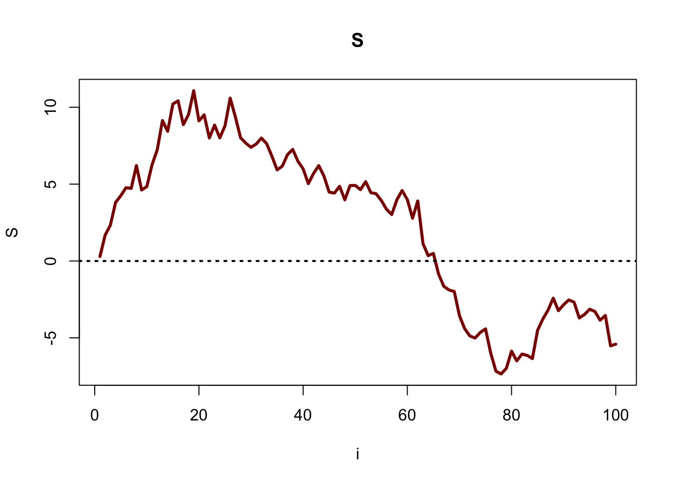
Let’s step through the code. The set.seed() function allows us to replicate our work. That is, computers are not truly random: they employ ‘pseudo-random’ processes, and ‘setting a seed’ allows us to generate the same ‘random’ process multiple times (see the Glossary for more).
The next bit of code , S = rep(NA, 100), sets up the path that we will fill with values (remember, it is often good practice to fill vectors with NA before filling them; again, see the Glossary for more).
Next, we need to define the first value with the code S[1] = rnorm(1, 0, 1). This value is slightly different from the rest of the values, because we know that \(S_{i - 1}\) in the case where \(i = 1\) is just \(S_0 = 0\), so we just have to generate a \(N(0, 1)\) draw to find \(S_1\).
Finally, we get to the loop. We have already filled in S[1], and we now have to fill in S[2] through S[100]. That means that we want i to increment from 2 to 100, which is why we have the code i in 2:100 in the for loop. From there, we generate \(S_i\). We do this by adding the previous value \(S_{i - 1}\) to a random draw from \(N(0, 1)\). Recall that \(i\) increments by 1 every time through the loop, so we work with S[i - 1] and S[i] in the code. For example, to find S[i] when i = 50, we add rnorm(1, 0, 1) to S[i - 1], which generates one random draw from a \(N(0, 1)\) and adds it to S[49].
The last line is simply a plot of our data; we will learn more about plotting in R later in this chapter.
While Loop
These are very similar to for loops, with one fundamental difference. A for loop runs a specific number of times while the index increments (usually, we use i for the index). A while loop runs ‘while a certain condition is satisfied.’ Consider this example:
#initialize i
i = 0

#the 'condition' is that i < 10
while(i < 10){

  #increment i
  i = i + 1

}

#print i
i
## [1] 10Here, we start and let i = 0. We then enter the loop, which states that we will run the loop as long as i is less than 10. Then, each time we run through the loop, we add 1 to i. Every time after we pass through the loop, we re-evaluate the condition in the loop to see if we will enter the body of the loop again. Clearly, we will stop the loop when i is equal to 10, since then i will not be less than 10, and thus the condition will be violated.
We could also use break in the loop to break out of the loop if we wanted; for example, if we satisfied the condition but still wanted to exit the loop, we could break out if we wanted. This could be useful if we wanted to sample X and Y to satisfy some condition; consider if we wanted to sample \(X, Y\) i.i.d. \(Unif(0, 1)\) such that \(X + Y < 1\) (again, see Chapter 4 for more background). One way to do this is by putting TRUE in the condition for the while loop (since TRUE is always TRUE, so the condition is satisfied), and then using break when we get a sample that satisfies the condition.
#replicate
set.seed(110)

#iterate until we break
while(TRUE){

  #draw X and Y
  X = runif(1)
  Y = runif(1)

  #see if we got the sample we wanted
  if(X + Y < 1){
    break
  }
}

#print X and Y
X + Y
## [1] 0.8326754Each pass through the loop, the ‘while’ marker checks if the condition is true, which, by construction, it is (we entered TRUE as the argument in the loop). We break out of the loop (with ‘break’) when we get a sample of X and Y such that X + Y < 1.
Graphics
The graphics included in the base package of R rank are useful and versatile. These plots are generally easy to create and produce attractive visuals for a variety of different purposes.
Plot()
The plot() function is the most generic, basic graphing function. We can create scatter plots, line graphs, etc., and we can customize these with a variety of different inputs. Consider the following plot:
#define vectors
x = 1:10
y = x^2

#create the plot
plot(x, y,
     main = "Our First Plot!",
     xlab = "x",
     ylab = "y",
     xlim = c(0, 10),
     ylim = c(0, 100),
     type = "l",
     lwd = 5,
     col = "darkred")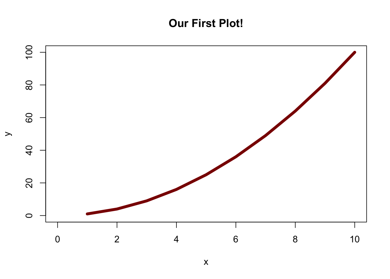
Let’s step through the code. Notice that we started a new line for each argument in the plot function, so that we (as humans) could more easily understand what’s going on. The first two (and most important) arguments are x and y, which tells the plot function to plot the x values vs. the y values (here, \(y = x^2\)).
The main argument dictates the title of the plot.
The xlab and ylab arguments dictate the x and y axes on the plot, respectively. Notice how for these arguments, as well as the main argument, we need to pass our title/axis label in quotation marks.
The xlim and ylim arguments determine the limits of the x and y axes. Notice how we have to bind the minimum and the maximum of the axes together with the c() function (again, short for ‘concatenate’).
The type argument dictates the type of graph. We use l here for a line graph, but we could use p for points, or even h for vertical bars.
The lwd argument dictates the width of the line. The larger the value, the thicker the line.
The col argument dictates the color of the line. See this database for an extensive palette of R colors.
Similar to the plot function, you can create histograms with the hist function. See the help page for more information, but many of the arguments are the same.
Plotting Techniques
There are a couple of interesting tools that help us expand on the basic plot function. First, consider the following code:
#plot on a 3x3 grid
par(mfrow = c(3,3))

#run the loop for the plots
for(i in 1:9){
  plot(rnorm(i*5),
       main = "",
       xlab = "x",
       ylab = "y",
       type = "p",
       pch = 16,
       col = "dodgerblue4")
}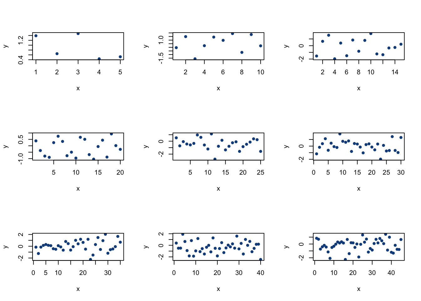
#restore the plot grid
par(mfrow = c(1,1))
The line par(mfrow = c(3,3)) tells R to plot on a 3x3 grid. The first plot we generate will be placed in the top left corner, the next graph in the top middle slot, etc. until all 9 slots have been filled in. Then, we ran a for loop (with a total of 9 iterations) that plotted values from a Normal distribution each time through the loop (with increasing sample sizes, as you can see on the plots). Make sure to restore the normal graphics state at the end with par(mfrow = c(1,1)) so R knows that we want to go back to the one plot grid.
We can also use the function abline to draw lines on plots that we create. Consider the following graphic.
#define vectors
x = seq(from = -10, to = 10, by = 1/10)
y = x^2

#plot
plot(x, y,
     main = "R Plot with Lines",
     xlab = "x",
     ylab = "y",
     type = "l",
     lwd = 4,
     col = "darkred",
     ylim = c(min(y), max(y)),
     xlim = c(-10, 10))

#draw lines
abline(v = 0,
       lwd = 2,
       col = "dodgerblue4")
abline(h = 40,
       lwd = 2,
       col = "dodgerblue4")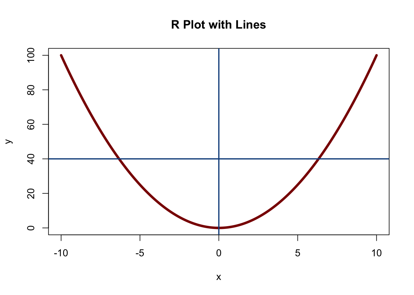
Here, we generated a plot, and then added two lines. The abline function is very similar to the plot function (i.e., it takes arguments like col and lwd), but the most important argument is the first one. Setting v = 5 as we did here means that we want to draw a vertical line at x = 5, and setting h = 8 means we want to draw a horizontal line at y = 8.
Glossary
Here, we provide a listing of common R functions, skills and techniques. You can reference this section whenever you see R syntax that you are unfamiliar with.
- Getting help in R. It’s usually very easy to get help about R functions, packages, etc. Simply type a question mark, followed by the thing you want help with, in the console, and a help window should pop up on the right (if you are working in RStudio).
?mean- Commenting in R. The pound sign,
#, is used to comment in English within a chunk of code so that, as a human reading the code, it is easier to understand what is going on (in general, it is very difficult to read code, especially someone else’s code!). R knows to skip over lines that start with the pound sign.
#This is a comment! R will not run this code.- Downloading packages/libraries. The base R package is full of useful features, but often you need to use something that is not included in the R base software. There are many useful tools in these extra ‘packages’ that we will need to install into R before we can do specific bits of work. To install a package that includes a bit of code that you might need, use the command
install.packages()and enter the package you want to install as your argument (within quotation marks!). You only need to install a package once. However, after a package is installed, you need to call that package when starting a session with the commandlibrary()(again, the package name is the argument, this time without quotations).
- Semi-colons. Use semi-colons in between chunks of code if you want R to print the output together.
#wihout a semi-colon
2 + 2
## [1] 42*2## [1] 4#with a semi-colon
2 + 2; 2*2## [1] 4## [1] 4- Arithmetic calculations (sum, mean, etc.). Many of these basic commands are built into R, and are very simple to use. We will get to this later, but the code
x = 1:3stores the vector \((1,2,3)\) inx.
#define a vector
x = 1:3

#find the sum, mean and standard deviation
sum(x); mean(x); sd(x)
## [1] 6## [1] 2## [1] 1TRUE, FALSER storesTasTRUEandFasFALSE, so it is bad practice to define anything asT(i.e., you shouldn’t create a vector and call itT; we will avoid this whenever possible calling the vector something else, likeX). Generally,TRUEandFALSEare used in conditions like ‘if’ statements.
#initialize x at 0
x = 0

#this should change x to 1
if(TRUE){
  x = 1
}

#print x
x
## [1] 1c(), or concatenation. Basically, this binds objects together.
#bind 1 and 2 into a vector
c(1, 2)
## [1] 1 2NA. This is short for ‘not available.’ Usually, we will fill a vector withNAbefore filling it. R cannot handleNAwhen doing calculations; for example, we couldn’t take the mean of a vector with anNAin it. This is why it is good practice to fill a vector withNAbefore filling it with our actual data; if we make a mistake and accidentally don’t fill a specific entry in the vector, R will let us know because we can’t even take a mean!
#fill a vector with ten NA entries
x = rep(NA, 10)

#fill the vector with 1 to 10, incrementing by 1
#   search 'for loops' and 'indexing' for more info
for(i in 1:10){
  x[i] = i
}set.seed(). There is no such thing as truly random number generation in a computer; the computer runs algorithms to generate ‘pseudo-random’ numbers. We can ‘set the seed’ of these algorithms to get the same results from ‘random’ processes, thus allowing us to replicate results when we come back and run the code again. For example:
set.seed(110)Now let’s try a random process; we’ll find the mean of 100 Standard Uniform random variables:
mean(runif(100))## [1] 0.5017964If we ran this again, since runif generates ‘random’ numbers, we get a different value:
mean(runif(100))## [1] 0.4751529However, if we ‘set the seed’ again (and we use the same seed, 110), we should get the same value as the first time we ran this:
set.seed(110)
mean(runif(100))
## [1] 0.5017964We’ll set seeds throughout these solutions to allow you to get the exact same results we did. The ‘seed’ will always be 110.
runif. This generates a set number of random draws,n, from an interval with a specified lower bound,min, and upper bound,max(i.e., from a \(Unif(a, b)\) random variable, where \(a\) is the min and \(b\) is the max). This is pretty standard across the ‘famous’ distributions we learn about; for example,rnormcan generate random values from a Normal distribution (therstands for random, and theunifmeans uniform, obviously). So, for example:
runif(n = 10, min = 0, max = 5)## [1] 1.9528672 0.4699530 3.4977928 4.6588981 1.1809279 1.9005877 2.3627924 0.7691976
## [9] 1.6524571 2.8443326Generates 10 random draws from 0 to 5. If you don’t include the min and max arguments…
runif(n = 10)## [1] 0.2836422 0.7407605 0.3658010 0.2006554 0.8325042 0.9261639 0.7242986 0.1317093
## [9] 0.2777294 0.5944356…the function defaults to the Standard Uniform with min of 0 and max of 1 (so a random draw from 0 to 1). This is a very useful way to ‘flip coins’ or simulate similar probabilistic events in R. For example, you could generate one value from a standard uniform; if it’s greater than .5, say that you got Heads, and if you got less than .5, say that you got Tails.
- ‘if’ statements, and/or logic. These are helpful logic statements that are pretty similar to other basic coding languages. Essentially, an ‘if’ command checks if a condition is true, and then, if it is true, it does something. For example:
#check if 1 equals 1
if(1 == 1){

  #set x equal to 10
  x = 10
}

#print x
x
## [1] 10This is saying ‘if 1 equals 1, then set x equal to 10.’ Since 1 does indeed equal 1, we see that x is now in fact 10. Notice some things about the syntax: we need two equals signs in the condition, the condition goes between the parentheses, and the ‘action’ (here setting x equal to 10) goes inside the curly braces.
We can further complicate this by adding ‘and’ and ‘or’ into our logical conditions as follows:
#see if 1 equals 2 OR 2 equals 2
if(1 == 2 || 2 == 2){
  x = 10
}


#see if 1 equals 2 AND 2 equals 2
if(1 == 2 && 2 == 2){
  x = 20
}

#print x
x
## [1] 10The first statement is saying ‘if 1 equals 2 OR 2 equals 2, set x = 10.’ The second is saying ‘if 1 equals 2 AND 2 equals 2, set x = 20.’ Clearly, the first is correct and the second is not correct, so x stores 10.
When we’re running a large chunk of code, we can incorporate ‘else’ and ‘else if’ statements, which are built with the same structure in mind.
- Random Variables. Most of the famous distributions we deal with have already been coded into R. We can easily generate random numbers from these distributions and work with their density functions. Take a look at the help pages of the following famous distributions to get a feel for them. Generally, functions that start with
r(i.e.,runif) generate random draws, functions that start withd(i.e.,dunif) return the density at a specific point, functions that start withp(i.e.,punif) return the CDF of a distribution up to a specific point, and functions that start withq(i.e.,qunif) return quantiles (i.e., the value at the \(50^{th}\) percentile of a distribution).
#Normal
?rnorm()

#Binomial/Bernoulli
?rbinom()

#Geometric
?rgeom()

#Exponential
?rexp()

#Beta
?rbeta()

#Gamma
?rgamma()

#Poisson
?rpois()

#Uniform
?runif()- rep. This creates a vector with specified length and specified values. For example:
x = rep(1, 5)Creates a vector that is 5 units long that we fill with 1’s, and stores it in x. We can index into the vector as follows:
x[3]## [1] 1This returns the 3rd value in the vector. This function will be very useful for setting up empty paths that we fill simulations with. We can also select against specific values in a vector.
x[-4]## [1] 1 1 1 1This returns every element in the vector x except the 4th element (it is tough to tell that we omitted the 4th element here, since every element is identical!).
matrix. This creates a matrix of data in R, where we can specify the valuesdata, the number of rowsnrowand columnsncol. For example, this command creates a 10 by 10 matrix of 0’s and calls itx.
x = matrix(data = 0, nrow = 10, ncol = 10)We can now access the \(i^{th}, j^{th}\) values of the matrix by indexing into it as follows:
x[4, 5]## [1] 0This grabs the element in the 4th row, 5th column of x (it is difficult to tell that we picked the correct value, since all of the values in this matrix are 0). This function will be very useful for setting up empty paths that we fill simulations with.
rbindandcbind. These stand for ‘row bind’ and ‘column bind.’ They take structures and bind them together by row or by column; this will be helpful when we work with multiple vectors or matrices.
#define two matrices
matrix0 = matrix(0, nrow = 3, ncol = 3)
matrix1 = matrix(1, nrow = 3, ncol = 3)

#bind by rows (top and bottom)
rbind(matrix0, matrix1)
## [,1] [,2] [,3]
## [1,] 0 0 0
## [2,] 0 0 0
## [3,] 0 0 0
## [4,] 1 1 1
## [5,] 1 1 1
## [6,] 1 1 1#bind by column (side by side)
cbind(matrix0, matrix1)## [,1] [,2] [,3] [,4] [,5] [,6]
## [1,] 0 0 0 1 1 1
## [2,] 0 0 0 1 1 1
## [3,] 0 0 0 1 1 1data.frame(in thedata.tablepackage). This converts some sort of data object, usually a matrix, into something called adata frame. For example:
#create the matrix
x = matrix(runif(20), nrow = 10, ncol = 2)

#convert to a data frame
x = data.frame(x)
Here, we create a matrix x with 10 rows and 2 columns (10 by 2) and filled it with 20 random draws from a uniform. Then, we change x to a ‘data.frame.’
One of the advantages of a data frame is that we can more easily perform certain key tasks on a specific type of object. For example, imagine if here we were collecting 10 data points for men and 10 for women (hence our 2 columns) and we wanted to find the mean for men. If we had a matrix, we would have to index into the matrix correctly; this is much easier with a data frame.
First, we can name the columns with the command colnames. The command rownames does the same thing, but for rows!
#name the columns
colnames(x) = c("Men", "Women")
Take a peek at x if you’d like; it should be the same as before, but with column names. Now we can grab those column names with the dollar sign operator:
#grab the 'Men' column
x$Men
## [1] 0.113263783 0.136841874 0.869321317 0.571819524 0.002760004 0.866104885 0.216270895
## [8] 0.738721495 0.557044378 0.441975039This grabs the vector of Men in our data frame. We can now perform all types of operations on it, like finding the mean for men:
mean(x$Men)## [1] 0.4514123We can also index into this in special ways. Imagine if we wanted to take the mean of the men’s results, but only when, on the same trial (same row), a women had a data point over .5. Then we would do:
mean(x$Men[x$Women > .5])## [1] 0.1368419Here, the code inside of the mean function returns the vector of Men within the data frame x; specifically, we index the values such that the corresponding value for Women is greater than .5.
unique. Returns the unique elements in a vector, which can be very useful in simulations; often we are interested in the length of the unique vector.
#define a vector
# remember, we use 'c()' to concatenate, or bind
vector1 = c("a", "a", "b", "c", "c", "d")

#there are 4 unique elements: "a", "b", "c" and "d"
unique(vector1)
## [1] "a" "b" "c" "d"length. Returns the length of an object, usually a vector. Very useful when we need to see how many values in a vector satisfy a certain condition.
#define this vector, which has 3 elements (length 3)
vector1 = c(5, 2, 4)
length(vector1)
## [1] 3#draw 10 values from a standard normal, count how many are negative
X = rnorm(10)
length(X[X < 0])## [1] 6In the bottom lines, we draw 10 values from a \(N(0, 1)\) random variable and store them in the vector X. The code X[X < 0] returns the subset vector of the vector X for which values of X are less than 0; we then find the length of this subset vector to count how many values of X are negative.
paste0. Essentially the same as the ‘concatenate’ function but also works with strings (i.e., objects made of text). Like thec()function, arguments are separated by commas.
#generate a random number
X = rnorm(1)

#print out a sentence
paste0("I generated the random number ", X, ".")
## [1] "I generated the random number -0.63180229621031."This is useful when we would like to print out the result of a random simulation, as we did above.
sample. This is an extremely useful function that simply samples from a desired vector. This is also a very versatile function. The first argument is the vector that we would like to sample from. From there, we can decide how many samples we would like to take (the second argument, calledsize), if we want to sample with or without replacement (the third argument, calledreplace), and the PMF of our sample (the fourth argument, calledprob).
#replicate
set.seed(110)

#generate a random iteration of the vector 1,2,...,5
sample(1:5)
## [1] 4 1 3 2 5#sample 3 values from the vector 1,2,...,5 without replacement
sample(1:5, 3)## [1] 1 4 3#sample 7 values from the vector 1,2,...,5 with replacement
sample(1:5, 7, replace = TRUE)## [1] 4 3 4 1 3 4 5#sample 7 values from the vector 1,2,...,5 with replacement
#and with a specific PMF
sample(1:5, 7, replace = TRUE, prob = c(.3, .3, .3, .1, 0))## [1] 2 2 3 3 3 4 3These examples show the sample function used with increasing complexity. If you do not specify the arguments replace and prob, the default is FALSE for replace (sample without replacement) and a uniform distribution for prob (sample each value with equal probability). In the final draw, we assigned a customized PMF by setting a vector for the ‘prob’ argument: this specifies that on each draw we should pick 1 with probability .3, 2 with probability .3, etc. Notice how we see a lot of 2’s and 3’s in this final draw, and no 5’s (since 5 has a probability of 0 of being selected, according to our defined PMF)
- The
:operator, used between numbers. This returns a vector with increments of size 1 between the two numbers.
#vector from 1 to 10, with steps of 1
1:10
## [1] 1 2 3 4 5 6 7 8 9 10#can also increment across numbers with decimals
4.7:8.7## [1] 4.7 5.7 6.7 7.7 8.7seq. Generates a sequence; we can decide where the sequence starts (with the first argumentfrom), where the sequence ends (with the second argumentto) and the size of the increments (either withby, which increments by a specific amount, orlength.out, which forces the sequence to be a specific length).
#create a vector from 1 to 10, increment by 1
seq(from = 1, to = 10, by = 1)
## [1] 1 2 3 4 5 6 7 8 9 10#create a vector from 20 to 30, with length 30
seq(from = 20, to = 30, length.out = 30)## [1] 20.00000 20.34483 20.68966 21.03448 21.37931 21.72414 22.06897 22.41379 22.75862
## [10] 23.10345 23.44828 23.79310 24.13793 24.48276 24.82759 25.17241 25.51724 25.86207
## [19] 26.20690 26.55172 26.89655 27.24138 27.58621 27.93103 28.27586 28.62069 28.96552
## [28] 29.31034 29.65517 30.00000round. This rounds a value (the first argument) to a specific decimal point (the second argument). This can be useful because R generates random values to many decimal places!
#round a random normal draw
round(rnorm(1), 2)
## [1] 0.97sort. Puts a vector (the first argument) in increasing or decreasing order (either set the second argument,decreasing, toFALSEorTRUE). The default is to return an increasing vector.
#create a vector
vector1 = c(1,2,3)

#sort the vector in two ways
sort(vector1)
## [1] 1 2 3sort(vector1, decreasing = TRUE)## [1] 3 2 1rev. Takes in a vector and returns the vector in reversed order.
#define a vector
vector1 = c(1,2,3)

#reverse it
rev(vector1)
## [1] 3 2 1- Indexing (square brackets:
[ ]). As we’ve seen, we can use square brackets to index into vectors. We can get a little more advanced by indexing into the vector and selecting all values that satisfy a certain condition.
#create a new vector from 1 to 5
x = 1:5

#select values in the vector that are less than 2
x[x < 2]
## [1] 1This selects all values in the vector x that satisfy the condition in the index: here, that the value is less than 2. We can complicate this function with R ‘and/or’ logic (notice here we only use one & in the indexing brackets).
x[x > 2 & x < 5]## [1] 3 4This selects all values in the vector x that are greater than 2 and less than 5.
- Graphics. The following commands help to generate useful, customizable graphics for R works. Try looking at the help pages to see how these functions work.
#standard plots
?plot

#histograms
?hist

#add another series to a plot
?lines

#add straight lines to a chart
?abline

#create a legend for a plot
?legendsapply. This is a very useful function that is often used in situations where ‘for loops’ are useful; it allows us to apply some function over a vector. Imagine if we had a large vectorXand we wanted to take the square of each value. We could usesapplyto apply the function (the function here is taking the square) over each value.
#generate a vector for X
X = rnorm(100)

#calculate the square of X
Y = sapply(X, function(x) x^2)
Here, the first argument in sapply is the function we want to iterate over, X. For the second argument, we write the function that we want to apply. We write this in the usual way we would define a function: function(x), followed by the function, which is x squared. It doesn’t matter that we used lowercase x; we could use any letter, as long as we are consistent!
Practice
Problems
0.1
There are 1.60934 kilometers in every mile. Write a function in R that converts kilometers to miles.
0.2
Show graphically that \(\frac{n!}{n!(n - k)!}\) where \(n! = n\cdot (n - 1)\cdot(n - 2)... \cdot 1\) (this is the binomial coefficient, which we discuss at length in Chapter 1) is maximized at \(k = n/2\) when \(n\) is even and \(k = \frac{n + 1}{2}, \frac{n - 1}{2}\) when \(n\) is odd.
0.3
Demren is wandering among the letters A to E. He starts at C and, every step, moves up or down a letter (i.e., from C he can go up to B or down to D) with equal probabilities (a 50/50 chance). Once he hits one of the endpoints A or E, he stops. Let \(X\) be the number of steps he takes. Using a simulation in R, estimate the mean and median of \(X\).
0.4
Imagine rolling a fair, six-sided die, and then flipping a fair, two-sided coin the number of times specified with the die (i.e., if we roll a 3, flip the coin 3 times). Let \(X\) be the number of heads you get in this experiment. Use a simulation in R to estimate the mean and median \(X\).