Chapter 5 Moment Generating Functions
“Statistics may be dull, but it has its moments” - Unknown
We are currently in the process of editing Probability! and welcome your input. If you see any typos, potential edits or changes in this Chapter, please note them here.
Motivation
We’ll now take a deeper look at Statistical ‘moments’ (which we will soon define) via Moment Generating Functions (MGFs for short). MGFs are usually ranked among the more difficult concepts for students (this is partly why we dedicate an entire chapter to them) so take time to not only understand their structure but also why they are important. Despite the steep learning curve, MGFs can be pretty powerful when harnessed correctly.
Moments and Taylor Series
Before we dive head first into MGFs, we should formally define statistical ‘moments’ and even freshen up on our Taylor Series, as these will prove especially handy when dealing with MGFs (and have likely already proven handy in the PMF problems of previous chapters).
The \(k^{th}\) moment of a random variable \(X\) is given by \(E(X^k)\). The ‘first moment,’ then, (when \(k=1\)) is just \(E(X^1) = E(X)\), or the mean of \(X\). This may sound like the start of a pattern; we always focus on finding the mean and then the variance, so it sounds like the second moment is the variance. However, the second moment is by definition \(E(X^2)\) (plug \(k = 2\) into \(E(X^k)\)). We know that \(E(X^2)\) is not quite the Variance of \(X\), but it can be used to find the Variance. That is, \(Var(X) = E(X^2) - E(X)^2\), or the Variance equals the second moment minus the square of the first moment (recall how LoTUS can be used to find both expectation and variance).
So, essentially, the moments of the distribution are these expectations of the random variable to integer powers, and often they help to give valuable information about the random variable itself (we’ve already seen how moments relate to the mean and variance). Since we’re such masters of LoTUS, we would be comfortable finding any specific moment for \(k>0\), in theory: just multiply \(x^k\), the function in the expectation operator, by the PDF or PMF of \(X\) and integrate or sum over the support (depending on if the random variable is continuous or discrete). This could take a lot of work, though (and we have to do a separate integral/sum for each distinct moment), and it’s here that MGFs are really valuable. After all, it’s in the name: MGFs are functions that generate our moments so we don’t have to do LoTUS over and over.
Let’s now briefly freshen up on our Taylor Series, because they are probably as rusty as they are important. We will see Taylor Series are closely related to calculating moments via an MGF, so it’s very important now to feel comfortable working with these series. Here are the chief examples that will be useful in our toolbox.
- The Exponential series:
\[e^x = 1 + x + \frac{x^2}{2!} + \frac{x^3}{3!} + ... = \sum_{n=0}^{\infty} \frac{x^n}{n!}\]
- Geometric series:
\[\frac{1}{1-x} = 1 + x + x^2 + x^3 + ... = \sum_{n=0}^{\infty} x^n\]
\[\frac{1}{(1 - x)^2} = 1 + 2x + 3x^2 + 4x^3 + ... = \sum_{n=0}^{\infty}nx^{n-1}\]
These hold for \(0 < x < 1\).
- Finally, less useful (for our purposes) but very easily recognizable, we have our Sin and Cos series.
\[sin(x) = x - \frac{x^3}{3!} + \frac{x^5}{5!} - \frac{x^7}{7!} + ... = \sum_{n=0}^{\infty}(-1)^n \frac{ x^{2n + 1}}{(2n + 1)!}\]
\[cos(x) = 1 - \frac{x^2}{2!} + \frac{x^4}{4!} - \frac{x^6}{6!} + ... = \sum_{n=0}^{\infty} (-1)^n \frac{x^{2n}}{(2n)!}\]
You can also find a handy, succinct guide for these Taylor Series and others here.
MGF Properties
Before we talk about what an MGF actually is, let’s talk about why it’s important. For now, just picture the MGF as some function that spits out moments. Let’s say that a random variable \(X\) has an MGF \(M(t)\) (that is, simply a function of a ‘dummy’ variable \(t\)). Here are a couple of reasons why the MGF \(M(t)\) is so special:
Property 5.1
If two random variables have the same MGF, then they must have the same distribution. That is, if \(X\) and \(Y\) are random variables that both have MGF \(M(t)\), then \(X\) and \(Y\) are distributed the same way (same CDF, etc.). You could say that the MGF determines the distribution. This is a neat result that could be useful when dealing with two unknown random variables. It’s also the same for PDFs/PMFs and CDFs; if two random variables have the same CDF or PDF/PMF (depending if they are discrete or continuous), then they have the same distribution.
Property 5.2
MGFs make dealing with sums of random variables easier to handle. For two random variables \(X\) and \(Y\), consider the sum \(X+Y\) (this is technically called a ‘convolution,’ which we will study in later chapters). If \(X\) and \(Y\) are independent, then there is a simple way to find the MGF of \(X + Y\): just multiply the separate, individual MGFs of \(X\) and \(Y\) (this will become more clear when we actually see what an MGF looks like). So, if \(X\) and \(Y\) are independent and \(X\) has MGF \(M_x(t)\) and \(Y\) has MGF \(M_y(t)\), then the MGF of \(X + Y\) is just \(M_x(t)M_y(t)\), or the product of the two MGFs.
Property 5.3
This is the key property, and proves the name of the MGF to be true: the \(n^{th}\) moment, \(E(X^n)\), of a distribution is the coefficient of \(\frac{t^n}{n!}\) in the Taylor Series of the MGF \(M(t)\). Mathematically, by the definition of a Taylor series, the \(n^{th}\) moment is also equal to the \(n^{th}\) derivative of \(M(t)\) evaluated at 0. This probably seems like a big step, but that’s because we haven’t even seen what an MGF looks like yet. Don’t worry too much thus far; the point here is that the MGF can generate the moments of a distribution (this ‘method’ is just how it generates them).
Now that we have established the relevance of the MGF (and perhaps been a little confusing along the way) we can formalize what the function actually looks like. For a random variable \(X\), we have that the MGF \(M(t)\), where \(t\) is a dummy variable, is defined:
\[M(t) = E(e^{tx})\]
It doesn’t look as menacing as you thought, right? This is a clear example of where LoTUS can be extremely useful; just multiply \(e^{tx}\), the function in the expectation operator, by the PDF of \(x\) and integrate/sum over the support to get the MGF of a random variable. Remember, \(t\) is just a placeholder that keeps track of the moments of the distribution; we’re going to end up plugging in different values of \(t\) to find different moments of the distribution.
It probably seems ridiculous to think that this simple expectation has the properties mentioned above. It certainly may seem pretty vague at the moment, and, as with other tricky concepts like Universality, it’s probably best to follow up with examples.
Using MGFs
Example 5.1 (Exponential MGF)
First, we’ll work on applying Property 6.3: actually finding the moments of a distribution. We’ll start with a distribution that we just recently got accustomed to: the Exponential distribution. This is a really good example because it illustrates a few different ways that the MGF can be applicable.
Let’s start by finding the MGF, of course. We’re going to use \(X \sim Expo(\lambda)\), and so the PDF is defined as \(\lambda e^{-x\lambda}\). The MGF, by definition, is just \(E(e^{tx})\), which we can just plug into a LoTUS calculation (multiply \(e^{tx}\) times the PDF of \(X\) and integrate over the support):
\[M(t) = \int_{0}^{\infty} e^{tx}\lambda e^{-x\lambda} dx = \lambda\int_{0}^{\infty} e^{-x(\lambda-t)} = -\lambda \frac{e^{-x(\lambda-t)}}{\lambda-t}\Big|_{0}^{\infty} = \frac{\lambda}{\lambda-t}\]
For \(t>0\) (this constraint is fine, because we don’t need to consider a ‘negative moment’).
Voila! This is the first MGF we’ve actually seen. Pretty simple, no? Notice here that \(\lambda\) is fixed, and \(t\) is what we are going to plug in to start to get the different moments (more about that in a second). Let’s confirm that this is in fact the MGF with a simulation in R. We will plot the analytical result above, as well as empirical estimates of \(E(e^{tx})\).
#replicate
set.seed(110)
sims = 1000

#define a simple parameter
lambda = 5

#generate the r.v.
X = rexp(sims, lambda)

#define t (in an interval near 0)
t = seq(from = 0, to = 2, length.out = 10)

#calculate the empirical and analytical MGFs
MGF.a = sapply(t, function(t) lambda/(lambda  - t))
MGF.e = sapply(t, function(t) mean(exp(t*X)))

#plot the MGFs, should match
plot(t, MGF.e, main = "Exponential MGF", xlab = "t",
     ylab = "", type = "l", col = "black", lwd = 3)
lines(t, MGF.a, type = "p", pch = 16,
      lwd = 3, col = "red")


legend("topleft", legend = c("Analytical MGF", "Empirical MGF"),
       lty=c(1,1), lwd=c(2.5,2.5),
       col=c("red", "black"))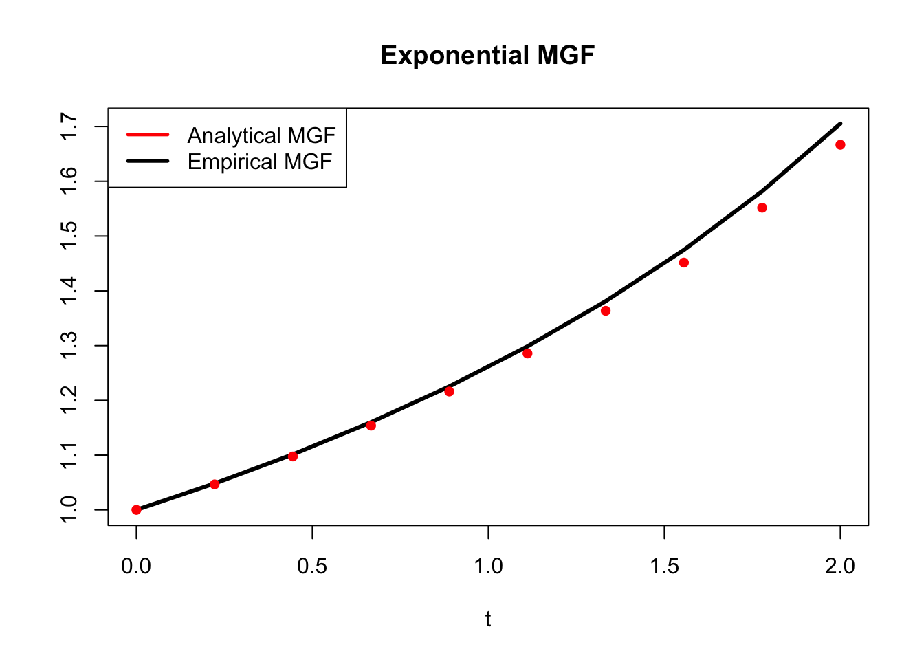
Now, what can we do with this MGF? Remember, for our purposes there are essentially two ways to get the moments from the MGF: first, you can take the \(n^{th}\) derivative and plug in 0 for the \(n^{th}\) moment. Second, you could find the coefficient for \(\frac{t^n}{n!}\) in the Taylor Series expansion.
That second one sounds a little vague, so let’s start with the derivatives. Say that we want the first moment, or the mean. We’ll just take the derivative with respect to the dummy variable \(t\) and plug in 0 for \(t\) after taking the derivative (remember how we said that \(t\) was a ‘dummy’ variable that would keep track of the moments? This is what was meant):
\[M'(t) = \frac{\lambda}{(\lambda - t)^2}, \; \; \; E(X) = M'(0) = \frac{\lambda}{\lambda^2} = \frac{1}{\lambda}\]
Incredibly, this is the correct mean of an \(Expo(\lambda)\) random variable. Let’s do the variance now; we already have the first moment, but we need the second moment \(E(X^2)\) as well. We can just derive again and plug in \(t= 0\) to find the second moment:
\[M''(t) = \frac{2\lambda}{(\lambda - t)^3}, \; \; \; E(X^2) = M''(0) = \frac{2\lambda}{\lambda^3} = \frac{2}{\lambda^2}\]
Now that we have our second moment, we can easily find the variance (remember, the second moment is not the variance, that’s a common misconception; we have to take the second moment minus the square of the first moment, by the definition of variance):
\[Var(X) = E(X^2) - E(X)^2 = \frac{2}{\lambda^2} - \frac{1}{\lambda^2} = \frac{1}{\lambda^2}\]
This exactly matches what we already know is the variance for the Exponential.
However, this seems a little tedious: we need to calculate an increasingly complex derivative, just to get one new moment each time. It’s quite useful that the MGF has this property, but it does not seem efficient (although it is probably more efficient than employing LoTUS over and over again, since derivation is easier than integration in general). Let’s try the second method of generating moments from the MGF: finding the coefficient of \(\frac{t^n}{n!}\) in the infinite series.
This seems ambiguous until you actually do it. We found that the MGF of the Exponential is \(\frac{\lambda}{\lambda - t}\). Does that look like any of the series we just talked about? Well, it does kind of look like a Geometric Series, but we have \(\lambda\) instead of 1. That’ s not a big deal, though, because we can recall our useful trick and let \(\lambda = 1\), which is just an \(Expo(1)\) (recall ‘scaling an Exponential’ from Chapter 4). Let’s try to work with that, then, since, like we have shown earlier, it’s pretty easy to convert into any other Exponential random variable.
Plugging in \(\lambda = 1\), we see that the MGF for an \(Expo(1)\) is \(\frac{1}{1- t}\), which is definitely a series that we have seen. In fact, expanded out, that’s just \(\sum_{n=0}^{\infty} t^n\) (see above).
So, we have \(t^n\) in the sum, but we know from our list of the ‘properties’ of the MGF that we need the coefficient not of \(t^n\) but of \(\frac{t^n}{n!}\). Can we fix that? Sure, if we just multiply by \(\frac{n!}{n!}\), we will get \(n!\frac{t^n}{n!}\), and then, clearly, the coefficient of \(\frac{t^n}{n!}\) is \(n!\) (this is a tricky step, so make sure that you go through it until it makes sense). So, the moments of the Exponential distribution are given by \((n!)\). That is, \(E(X^n) = n!\), in general.
Let’s do a quick check. We know that the mean and the variance of an \(Expo(1)\) are both 1, so this should match up with what we’ve just found. Well, the mean is first moment, and plugging \(n=1\) in to \(n!\), we get 1, so that checks out. The variance is the second moment minus the first moment squared, and the second moment is \(n=2\) plugged in to \(n!\), or 2. So, we just do \(2 - 1^2 = 1\), which is the variance, and this checks out.
We could always convert back to any Exponential distribution \(X \sim Expo(\lambda)\). Remember, if \(\lambda X = Y\), then \(Y \sim Expo(1)\), and we already have a very good way to find the moments for this distribution. We could turn this into finding the moments of \(X\) very easily:
\[(\lambda X)^n = Y^n \rightarrow \lambda^n X^n = Y^n \rightarrow X^n = \frac{Y^n}{\lambda^n}\]
And then we could just take the expected value of both sides:
\[E(X^n) = E(\frac{Y^n}{\lambda^n}) = \frac{E(Y^n)}{\lambda^n}\]
Remember, \(E(X^n)\) is just the \(n^{th}\) moment, and we know that the \(n^{th}\) moment of \(Y\) is just \(n!\), so we can plug in \(n!\) for \(E(Y^n)\):
\[E(X^n) = \frac{n!}{\lambda^n}\]
And we have a nice, closed form way to find the moments for any Exponential distribution, which is much faster and easier than computing the LoTUS integral every time.
Additionally, it’s clear that this is even a much cleaner and, in the long run, easier way to find moments than using the MGF to take derivatives over and over again. Instead of taking 10 derivatives, for example, we could just plug in \(n=10\) to that expression that we got; it’s much simpler. So, remember that often a really nice way to get moments is just to expand the MGF into a sum and find the coefficient of \(\frac{t^n}{n!}\).
Example 5.2 (Sum of Poissons):
Let’s now try to synthesize Property 5.1 and Property 5.2. Let \(X\) and \(Y\) be i.i.d. \(Pois(\lambda)\) random variables. Consider the distribution of \(Z\), where \(Z = X + Y\). We know by the story of a Poisson that \(X\) and \(Y\) are both ‘counting the number of winning lottery tickets in a lottery with rate parameter \(\lambda\)’; that is, we have many trials, with low probability of success on each trial. What do we expect to be the distribution of ‘combining’ these two lotteries?
You may have some intuition for this problem, but a little bit of work with MGFs can help to solidify this intuition (as well as our understanding of MGFs). Specifically, what we can do is find the MGF of \(Z\), and see if it matches the MGF of a known distribution; if they match, by Property 5.1, then they have the same distribution and we thus know the distribution of \(Z\). We can find the MGF of \(Z\) by Property 5.2: find the individual MGFs of \(X\) and \(Y\) and take the product.
So, let’s get to work finding the MGF of \(X\). We write out the LoTUS calculation, where \(M_x(t)\) denotes the MGF of \(X\):
\[M_x(t) = E(e^{tx}) = \sum_{k = 0}^{\infty} e^{tk} \frac{\lambda^k e^{-\lambda}}{k!}\]
We can take out the \(e^{-\lambda}\) because it doesn’t change with the index \(k\).
\[e^{-\lambda} \sum_{k = 0}^{\infty} e^{tk} \frac{\lambda^k }{k!}\]
We can then combine terms that are raised to the power of \(k\):
\[= e^{-\lambda} \sum_{k = 0}^{\infty} \frac{(e^t \lambda)^k }{k!}\]
Now recall the Exponential series that we mentioned earlier in this chapter. The sum looks like the expansion of \(e^{e^t \lambda}\), so we write:
\[= e^{-\lambda}e^{e^t \lambda}\] \[= e^{e^t \lambda - \lambda}\] \[= e^{\lambda(e^t - 1)}\]
This is the MGF of \(X\), which is \(Pois(\lambda)\). It may look a little strange, because we have the \(e\) in the exponent of the \(e\). We know that, since \(Y\) has the same distribution as \(X\), it has the same MGF (by Property 5.1), so the MGF of \(Y\) is also \(= e^{\lambda(e^t - 1)}\) (both are functions of the ‘bookkeeping’ variable \(t\)). By Property 5.2, we take the product of these two MGFs (which are identical) to find the MGF of \(Z\). Letting \(M_z(t)\) mean ‘the MGF of \(Z\)’:
\[M_z(t) = e^{\lambda(e^t - 1)}e^{\lambda(e^t - 1)}\] \[ = e^{2\lambda(e^t - 1)}\]
What about this MGF is interesting? Note that it has the exact same structure as the MGF of a \(Pois(\lambda)\) random variable (i.e., the MGFs of \(X\) and \(Y\)) except it has \(2\lambda\) instead of \(\lambda\). The implication here is that \(Z \sim Pois(2\lambda)\), and this must be true by Property 5.1 because it has the MGF of a \(Pois(2 \lambda)\) (imagine substituting \(2\lambda\) in for \(\lambda\) for the MGF of \(X\) calculation). We can quickly confirm this result by comparing the sum of two \(Pois(1)\) random variables to a \(Pois(2)\) random variable in R.
#replicate
set.seed(110)
sims = 1000

#generate the r.v.'s
X = rpois(sims, 1)
Y = rpois(sims, 1)
Z = rpois(sims, 2)

#set a 1x2 grid
par(mfrow = c(1,2))

#graphics; histograms should match (match the break)
hist(X + Y, main = "X + Y", xlab = "",
     col = rgb(1, 0, 0, 1/4), breaks = 0:10)
hist(Z, main = "Z", xlab = "",
     col = rgb(0, 1, 0, 1/4), breaks = 0:10)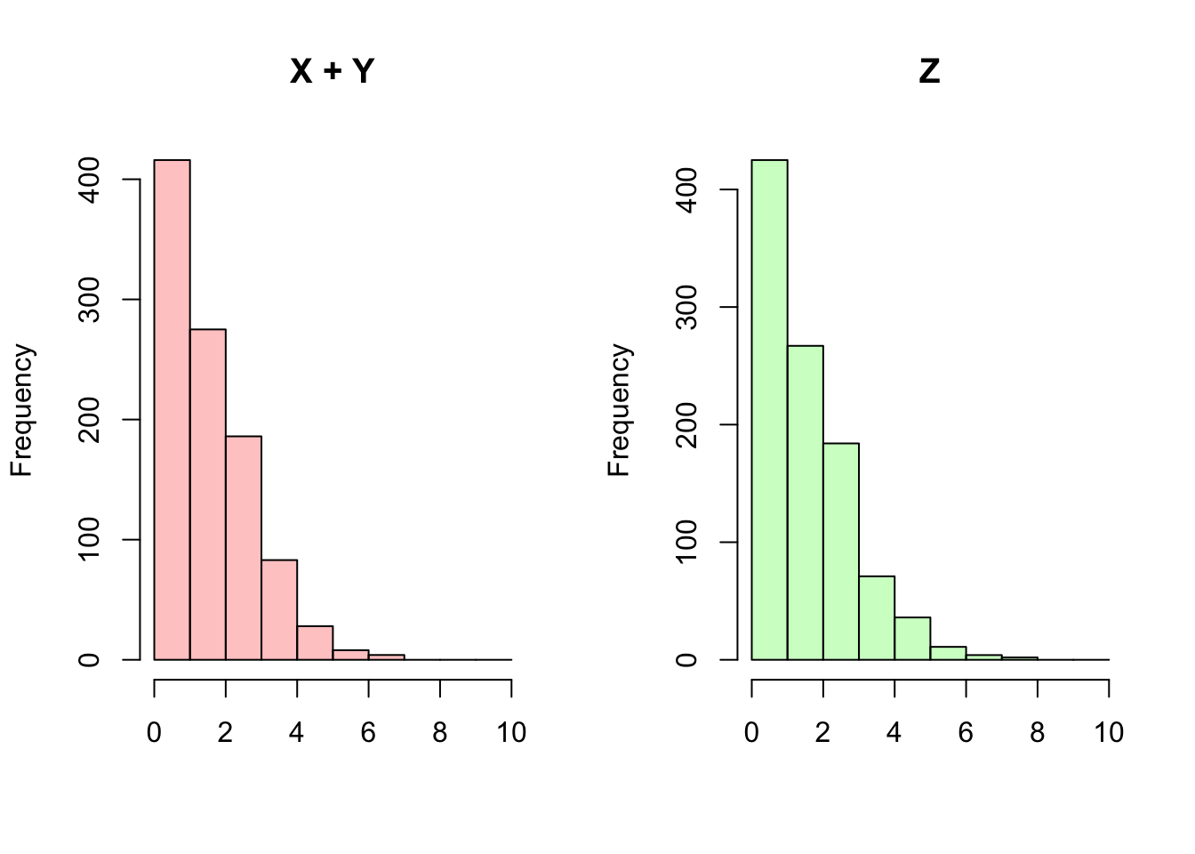
#re-set graphics
par(mfrow = c(1,1))
Ultimately, we have proven that the sum of Poisson random variables is Poisson, and even have shown that the parameter of this new Poisson is the sum of the parameters of the individual Poissons. This result probably matches your intuition: if we are considering the sum of the number of successes from two ‘rare events’ (i.e., playing both lotteries) we essentially have another ‘rare event’ with the combined rate parameters (since we are ‘in’ both lotteries). That is, the story of the Poisson is preserved.
Hopefully these were helpful examples in demonstrating just what MGFs are capable of doing: finding the moments of a distribution in a new and unique way (well, two ways actually), and learning more about specific distributions in general. Don’t be scared by the ugly integration and summations; usually things will work out cleanly and you will get a tractable expression for the moments of a distribution you’re interested in. MGFs really are extremely useful; imagine if you were asked to find the \(50^{th}\) moment of an \(Expo(\lambda)\). That sounds like an ugly LoTUS integral, but sounds very doable using the MGF approaches we’ve established.
Practice
Problems
5.1
We have discussed how a Binomial random variable can be thought of as a sum of Bernoulli random variables. Using MGFs, prove that if \(X \sim Bin(n, p)\), then \(X\) is the sum of \(n\) independent \(Bern(p)\) random variables.
Hint: The Binomial Theorem states that \(\sum_{k = 0}^n {n \choose k} x^n y^{n - k} = (x + y)^n\).
5.2
Ulysses has been studying the Uniform distribution and he makes the following claim. ‘Let \(X \sim Unif(0, 10)\) and \(Y_1, Y_2, ..., Y_{10}\) be i.i.d. \(Unif(0, 1)\). The sum of the \(Y\) random variables \(\sum_{k = 1}^{10} Y_k\) has the same distribution as \(X\); this is intuitive, adding up 10 random draws from 0 to 1 is the same as generating one random draw from 0 to 10.’ Test Ulysses’ claim using MGFs.
Defend your answer to (a.) using intuition.
5.3
Let \(X\) be a degenerate random variable such that \(X = c\) always, where \(c\) is a constant. Find the MGF of \(X\), and use the MGF to find the expectation, variance and all moments of \(X\). Explain why these results make sense.
5.4
Let \(X \sim N(\mu, \sigma^2)\). The MGF of \(X\) is given by \(M_x(t) = e^{\mu t + \frac{1}{2} \sigma^2 t^2}\) (in general, you can find this and other useful facts about distributions on Wikipedia). Using this fact, as well as properties of MGFs, show that the sum of independent Normal random variables has a Normal distribution.
5.5
Let \(X \sim Expo(\lambda)\) and \(Y = X + c\) for some constant \(c\). Does \(Y\) have an Exponential distribution? Use the MGF of \(Y\) to answer this question.
BH Problems
The problems in this section are taken from Blitzstein and Hwang (2014). The questions are reproduced here, and the analytical solutions are freely available online. Here, we will only consider empirical solutions: answers/approximations to these problems using simulations in R.
BH 6.13
A fair die is rolled twice, with outcomes \(X\) for the first roll and \(Y\) for the second roll. Find the moment generating function \(M_{X+Y}(t)\) of \(X+Y\) (your answer should be a function of \(t\) and can contain un-simplified finite sums).
BH 6.14
Let \(U_1, U_2, ..., U_{60}\) be i.i.d.~\(Unif(0,1)\) and \(X = U_1 + U_2 + ... + U_{60}\). Find the MGF of \(X\).
BH 6.21
Let \(X_n \sim Bin(n,p_n)\) for all \(n \geq 1\), where \(np_n\) is a constant \(\lambda > 0\) for all \(n\) (so \(p_n = \lambda/n\)). Let \(X \sim Pois(\lambda)\). Show that the MGF of \(X_n\) converges to the MGF of \(X\) (this gives another way to see that the Bin(\(n,p\)) distribution can be well-approximated by the \(Pois(\lambda)\) when \(n\) is large, \(p\) is small, and \(\lambda = np\) is moderate).