Chapter 8 Beta and Gamma

“It is likely that unlikely things should happen.” - Aristotle

We are currently in the process of editing Probability! and welcome your input. If you see any typos, potential edits or changes in this Chapter, please note them here.

Motivation

While the title sounds like this chapter prefaces an introductory discussion of the Greek alphabet, this section will actually cover two of the more confusing distributions in this book. Historically, students have had relatively more trouble with the Beta and Gamma distributions (compared to other distributions like the Normal, Exponential, etc.), which is unfortunate because of their valuable applications in theoretical probability and beyond. Hopefully a close look at the mechanics behind the two distributions will yield a deeper understanding of the Beta and Gamma.

Beta

We’ve often tried to define distributions in terms of their stories; by discussing what they represent in practical terms (i.e., trying to intuit the specific ‘mapping’ to the real line), we get a better grasp of what we’re actually working with. It helps to think of the Binomial as a set number of coin flips, or the Exponential as the time waiting for a bus. The issue with the Beta that likely contributes to its ‘aura of difficulty’ is that it doesn’t necessarily have a ‘cute,’ simple story that helps to define it. Again, you could think of the Poisson as the number of winning lottery tickets, or the Hypergeometric as drawing balls from a jar, but there’s really not any extremely relevant real-world connections for the Beta. Instead, probably the most common story for the Beta is that it is a generalization of the Uniform.

That sounds a little strange. What exactly is a generalization of a distribution? Well, let’s first consider the Uniform distribution itself. The Uniform is interesting because it is a continuous random variable that is also bounded on a set interval. Think about this for a moment; the rest of the continuous random variables that we have worked with are unbounded on one end of their supports (i.e., a Normal can take on any real value, and an Exponential can go up to infinity). The Uniform, as we know, has a bounded interval, often between 0 and 1 (the Standard Uniform). The Beta, in turn, is also continuous and always bounded on the same interval: 0 to 1. However, it is (usually) not flat or constant like the Uniform. That’s where the ‘generalization’ comes in: it shares these key properties (continuous and bounded) but is generalized to different shapes (not just flat like the Uniform).

In fact, in general, the Beta does not take on any one specific shape (recall that the Normal is bell-shaped, the Exponential right-skewed, etc.). Changing the parameters \((a,b)\) (which you might also see as \(\alpha\) or \(\beta\), and are the two parameters that the Beta takes, like the Normal takes \(\mu\) and \(\sigma^2\)) actually changes the shape of the distribution drastically. For example, if you allow \(a=b=1\), then you get a Standard Uniform distribution. If \(a=b=2\), you get a smooth curve (when you generate and plot random values). You can manipulate the shape of the distribution of the Beta just by changing the parameters, and this is what makes it so valuable. Remember, though, that no matter the shape, the Beta i continuous and is always bounded between 0 and 1 (the support is all values from 0 to 1).

Now that we have sort of an idea of what the Beta looks like (or, more importantly, has the potential of looking like, since we know that it can change shape) let’s look at the PDF. Remember that, like the Uniform, the Beta has two parameters \(a\) and \(b\) (often called \(\alpha\) and \(\beta\)). If \(X \sim Beta(a,b)\), the PDF is given by:

\[f(x) = \frac{\Gamma(a+b)}{\Gamma(a)\Gamma(b)}x^{a-1}(1-x)^{b-1}\]

Where \(\frac{\Gamma(a+b)}{\Gamma(a)\Gamma(b)}\) is just the normalizing constant that allows this to be a valid PDF; i.e., allows the function to 1 over the support (we’ll talk about what \(\Gamma\) means later. It’s just the ‘Gamma function,’ which of course we will see later in the chapter. Don’t worry about it for now). We’re going to more rigorously discuss this normalizing constant later in the chapter; for now, just understand that it’s there to keep this a valid PDF (otherwise the PDF would not integrate to 1).

You can already see how changing the parameters drastically changes the distribution via the PDF above. For example, we said before that if \(a=b=1\) we get a Uniform. That is, if we plug in 1 for both \(a\) and \(b\), the \(x\) and \(1 - x\) terms go away and we are left with a constant, which is indeed the PDF of a Standard Uniform (recall that, intuitively, it is a constant and thus doesn’t change with \(x\)). If we set \(a\) and \(b\) to 2, our \(x\) terms simplify to \((x-x^2)\), or a smooth curve, as mentioned above. The point is that this PDF can change drastically based on the parameters in question, which is what we identified as the chief characteristic of the Beta.

The expected value of a Beta is just \(\frac{a}{a+b}\), and the Variance is a bit more complex; it’s usually written in terms of the Expectation. You can find it on William Chen and Professor Blitzstein’s probability cheatsheet; we won’t really discuss it here because it doesn’t help a ton with intuition.

You can further familiarize yourself with the Beta with our Shiny app; reference this tutorial video for more.

Click here to watch this video in your browser. As always, you can download the code for these applications here.

Priors

It’s probably good to talk about why the Beta is so important now, since it doesn’t look very valuable at the moment. In fact, you can think about this section as kind of another story for the Beta: why it’s important and applied in real world statistics (kind of like how one of the stories for the Normal is that it’s the asymptotic distribution of the sum of random variables, by the Central Limit Theorem, which we will formalize in Chapter 9).

The Beta wears many hats, and one is that it is a conjugate prior for the Binomial distribution. ‘Conjugate priors’ are very important in more inferential applications, and you will become very familiar with this topic if you continue on your path of Statistics. Here, it’s probably best to start from scratch (we don’t even know what a prior is yet, let along a conjugate prior). It’s tough to formalize the definition without going through an example, so that is just what we will do.

Say that you were interested in polling people about whether or not they liked some political candidate. The people’s opinions are independent, they can only say yes or no, and we assume that there is a fixed probability that a random person will say ‘yes, I like the candidate.’ Therefore, we can assume that \(X\), the number of people that like the candidate, is a Binomial such that \(X \sim Bin(n,p)\) where \(n\) is the number of people you interview and \(p\) is the probability that each one says yes (we also believe that the population we sample from is large enough that we are essentially sampling with replacement; that is, taking one person out of the large population doesn’t change the population makeup in any significant way). You can also think of \(p\) as the expected proportion of the votes that the candidate gets (if a random person has probability \(p\) of voting yes, then we expect a fraction \(p\) of people to vote yes).

However, and you probably have wondered this before, we don’t really know what \(p\) is! We can estimate it, or even have a couple of our friends make guesses at it, but we’re not totally sure what the true probability is that someone says yes. So, essentially, we are dealing with an uncertainty about the true probability, and in ‘Bayesian’ statistics (recall Bayes’ Rule, same guy) we deal with that uncertainty by assigning a distribution to the parameter \(p\); that is, we make \(p\) a random variable that can take on different values because we are unsure of what value it can take on. This is called a prior distribution on our parameter, \(p\). This is interesting because we’re taking a parameter, which we have assumed to be a fixed constant up to this point (i.e., \(\mu\) for a Normal distribution, which we’ve said to be a constant), and allowing it to be a random variable.

To think of a concrete example, you could picture yourself assigning a Normal distribution to \(p\). Maybe you think that on average 60\(\%\) of people will say yes, so perhaps \(p \sim N(.6,.1)\) or something else centered around .6 (the .1 selection for variance is arbitrary in this case; in the real world, there are all sorts of different method for choosing the correct parameters). That’s the idea: to make \(p\) a random variable to reflect our uncertainty about it.

This is where the Beta comes in. We gave the Normal distribution as an example for the prior simply because we are very familiar with it; however, it is probably clear why the Normal distribution is not the best choice for a prior here. The support of a Normal distribution covers all real numbers, and no matter how small you make the variance, there will always be a chance that the random variable takes on a value less than 0 or greater than 1. Of course, we are working with a probability, \(p\), which we know must be between 0 and 1, so these cases are troublesome.

So, we would like to bound our probability, and a continuous random variable would probably also be nice in this case (since \(p\), what we are interested in, is a probability and is thus continuous: it can take on any value between 0 and 1). Do any distributions come to mind? Well, what about the Beta? We know that it’s the only bounded continuous distribution that we’ve learned (besides the Uniform) so it will work well for us here. In fact, this is one of the Beta’s chief uses: to act as a prior for probabilities, because we can bound it between 0 and 1 and shape it any way we want to reflect our belief about the probability. Certain that \(p\) is around .6? Concentrate the Beta around there. Not so certain? Flatten the Beta out, all by simply adjusting the parameters. This gives the Beta an advantage over the other bounded continuous distribution that we know, the Uniform: this distribution is flat and unchanging across a support.

For our prior, then, we will say that \(p \sim Beta(a,b)\). Since we have just assigned a prior to \(p\) and therefore made it a random variable, we can now think about \(X\), the total number of people that say yes, conditioned on \(p\). That is, based on whatever value our random variable \(p\) takes on, \(X\) is a Binomial with that probability parameter. If \(p\) takes on .7, then \(X \sim Bin(n,.7)\). If \(p\) takes on .55, then \(X \sim Bin(n,.55)\). You get the idea. In the end, we can say \(X|p \sim Bin(n,p)\) (recall our discussion of conditional distributions from Chapter 6).

This is a logical set-up so far, and the next step is to find the posterior distribution of \(p\). That is, how do we update our beliefs about \(p\) based on the data that we observe? For example, if 80\(\%\) of people answer yes to our question in a survey, that gives us information about \(p\) (intuitively, our best guess is that \(p\) is around \(80\%\)). If only \(40\%\) answer yes, that gives us information that \(p\) might be less than \(1/2\); you get the point. What we’re really looking for is the distribution of \(p|X\), or the distribution of the probability that someone votes yes given what we saw in the data (how many people we actually observed voting yes). In our notation, this is just \(f(p|X=x)\); that is, the PDF of \(p\) conditioned on \(x\) people saying ‘yes.’

From here, using Bayes Rule (recall that this is a common approach in ‘Bayesian’ Statistics), we know that:

\[f(p|X=x) = \frac{P(X=x|p)f(p)}{P(X=x)}\]

Before we calculate this, there is something we have to keep in mind: we are concerned about the distribution of \(p\), so we don’t have to worry about terms that aren’t a function of \(p\). This sounds strange, but bear with it for now.

Based on this ‘ignore non-\(p\) terms’ hint, we can ignore \(P(X = x)\). We’re interested in \(f(p|x)\) as a function of \(p\), so \(P(X = x)\) is a constant (because it is the marginal PMF of \(X\) and thus does not include \(p\) terms; recall that we marginalize out unwanted variables to get PMFs solely in terms of the random variable of interest). Instead, we can drop the \(P(X = x)\) and replace the \(=\) sign with \(\propto\), the proportionality sign. If you’ve never seen the proportionality sign before, you might use it for something like this: \(y \propto 2y\). No matter what value of \(y\) we have, the left side will be half of the right side (they are proportional by a factor of 2); in general, we could write a similar expression for any constant (not just 2). Anyways, since \(P(X= x)\) is a constant in our case, we have:

\[f(p|x) \propto P(X = x|p)f(p)\]

We know \(f(p)\), since this is simply the marginal PDF of a Beta with parameters \(\alpha\) and \(\beta\). We know \(P(X = x|p)\), since \(X\) conditional on \(p\) is \(Bin(n,p)\), so \(P(X = x|p)\) is the PMF of a Binomial with parameters \(n\) and \(p\).

\[f(p|x) \propto \Big({n \choose x}p^x q^{n-x}\Big) \Big(\frac{\Gamma(\alpha + \beta)}{\Gamma(\alpha)\Gamma(\beta)}p^{\alpha - 1} q^{\beta - 1}\Big)\]

Combining terms:

\[f(p|x) \propto \Big({n \choose x}\frac{\Gamma(\alpha + \beta)}{\Gamma(\alpha)\Gamma(\beta)}\Big) \Big(p^{x + \alpha - 1} q^{n - x+ \beta - 1}\Big)\]

Again, everything that is not a function of \(p\) is a constant that can be ignored, and we maintain proportionality:

\[f(p|x) \propto p^{x + \alpha - 1} q^{n - x+ \beta - 1}\]

Recall that \(p\) is our random variable; amazingly, this PDF looks like a PDF that we know. In fact, it looks like the PDF of a Beta (again, without the normalizing constant, but we don’t really care about this for determining a distribution. We still can identify the distribution, even if we don’t see the normalizing constant!). So, we can say with full confidence that, conditioning on how many people we actually saw say ‘yes’:

\[p|X= x \; \sim \; Beta(\alpha + x, \beta + n - x)\]

We can check this result with a simulation in R, where we generate \(p\) from the prior distribution and then generate \(X\) conditioned on this specific value of \(p\). We should see that, conditioned on \(X\) being some value, the density of \(p\) matches the analytical density we just solved for (that is, it has a Beta distribution with the above parameters).

#replicate
set.seed(110)
sims = 1000

#define simple parameters
#Beta(1, 1) is uniform, which is a good place to start if we are unsure about p
alpha = 1
beta = 1
n = 10

#generate the r.v.'s
p = rbeta(sims, alpha, beta)
X = sapply(p, function(x) sum(rbinom(1, n, x)))


#condition on a specific value of x
x = 7

#graphics; should match
plot(density(p[X == x]), main = "PDF of p|X = 7",
     xlab = "p", lwd = 3, col = "black", 
     ylim = c(0, 3), xlim = c(0, 1))

lines(seq(from = 0, to = 1, length.out = 100), dbeta(seq(from = 0, to = 1, length.out = 100), alpha + x, beta + n - x), lwd = 3, col = "red")

legend("topleft", legend = c("Empirical PDF", "Analytical PDF"),
       lty=c(1,1), lwd=c(2.5,2.5),
       col=c("black", "red"))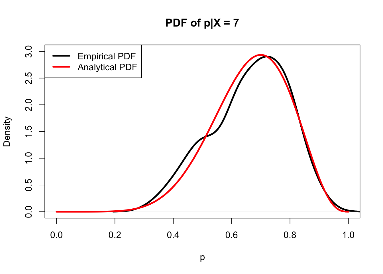

To actually apply this result in a real-world context (recall that we started by considering polling people about their favorite politicians) we would collect the data and observe \(X = x\), and then determine your distribution for \(p\). Here it looks like \(x\) is the number of successes, so basically you have a Beta with parameter \(a\) plus number of successes and \(b\) plus number of failures. It’s tough to mentally envision what the Beta distribution looks like as it changes, but you can interact with our Shiny app to engage more with Beta-Binomial Conjugacy. Reference this tutorial video for more; there is a lot of opportunity to build intuition based on how the posterior distribution behaves.

Click here to watch this video in your browser. As always, you can download the code for these applications here.

Anyways, the neat thing here was that we used a Beta distribution as our prior for \(p\), and it just so happened that, after all of the algebra, the posterior distribution for \(p\) was also Beta (again, updated based on the number of successes that we actually saw). This is the definition of a conjugate prior: when a distribution is used as a prior and then also works out to also be the posterior distribution (that is, conjugate priors are types of priors; you will often use priors that are not conjugate priors!). It’s another reason why we like the Beta: because it has this nice, clean property of working out to be the posterior distribution for \(p\) (at least with the Binomial; the Beta is not necessarily a conjugate prior for other distributions). This is a big reason why the Beta is popular and so often used in real life, since it’s such a good way to model probabilities that we are uncertain about in the real world. It’s pretty interesting that the above process yielded us a distribution for \(p\), which allows us to make all sorts of statements about this unknown parameter.

Order Statistics

The Beta allowed us to explore prior and posterior distributions, and now we will discuss a new topic within the field: Order Statistics. As we’ll see, these are essentially ‘ranked’ random variables.

Consider a set of random variables \(X_1, X_2, ..., X_n\). For concreteness, you might assume that they are all i.i.d. Standard Normal; however, this is not a requirement (we simply need \(n\) total random variables, they do not have to be independent or even from the same distribution). Now, define the \(j^{th}\) order statistic (which we will denote \(X_{(j)}\)) as the \(j^{th}\) smallest random variable in the set \(X_1, X_2, ..., X_n\). The term ‘\(j^{th}\) smallest’ is a bit tricky; think about this in specific cases. For example, \(X_{(1)}\) is the first order statistic, or the smallest of \(X_1, X_2, ..., X_n\) (you could more succinctly say \(X_{(1)} = min(X_1, X_2, ..., X_n)\)). We then have that \(X_{(2)}\), the second order statistic, is the second-smallest of \(X_1, X_2, ..., X_n\). We continue in this way until we get to the \(n^{th}\) order statistic, or the maximum of \(X_1, X_2, ..., X_n\).

It helps to step back and think about this at a higher level. Recall that a function of random variables is still a random variable (i.e., if you add 3 to a random variable, you just have a new random variable: your old random variable plus 3). Here, we do have random variables \(X_1, X_2, ..., X_n\), and we do apply a function (in the case of \(X_{(1)}\), or the first order statistic, we apply the ‘minimum’ function). You could also think about the official definition of statistic: a function of the data. Here, we can consider the data to be \(X_1, ..., X_n\), and we have a function that ranks them (i.e., we might try to find the minimum, or the second smallest, or third smallest, etc.).

Consider now a simple case where \(X_{1}, X_{2}\) are i.i.d. \(N(0, 1)\) random variables. We can envision a case where \(X_1\) crystallizes to -1 and \(X_2\) crystallizes to 1. In this case, \(X_{(1)}\), the first order statistic, is -1 (the minimum of \(X_1\) and \(X_2\)) and the second order statistic \(X_{(2)}\) is 1. The name ‘order statistic’ makes sense, then; we are ordering our values and assigning order statistics based on their rank!

In this specific example with Standard Normals, \(X_{(1)}\), the first order statistic, is the random variable that crystallizes to the maximum of two draws from a Standard Normal. Similarly, \(X_{(2)}\) is simply the minimum of two draws from a Standard Normal. We know that, with probability \(1/2\), \(X_{(1)}\) will be equal to \(X_1\) (since, by symmetry, there is a \(1/2\) probability that \(X_1 < X_2\) and thus \(X_1 = min(X_1, X_2) = X_{(1)}\)), and with probability \(1/2\) will be equal to \(X_2\) (by symmetry, \(X_{(2)}\) has the same structure). We know that \(X_{(1)} + X_{(2)}\) is always equal to \(X_1 + X_2\), since if \(X_{(1)}\) is equal to \(X_1\) or \(X_2\), then \(X_{(2)}\) must be equal to the other (i.e., if \(X_{(1)} = X_2\), then \(X_{(2)} = X_1\)). We also know that \(X_{(1)}\) and \(X_{(2)}\) are dependent; if we know that \(X_{(1)} = 0\), for example, then we know that \(X_{(2)}\) must be greater than 0 (since it is the maximum, and the minimum is 0).

We mentioned above that \(X_1, X_2,...,X_n\) can be any random variables (dependent, different distributions, etc.), but for our purposes we will consider i.i.d., continuous random variables. There are a couple of reasons for this simplification. First, i.i.d. is simply an easier case to deal with than random variables that are dependent or have different distributions. Second, discrete random variables have probabilities of ties when we try to order them. That is, if we have that \(X_1, X_2\) are i.i.d. \(Bern(1/2)\) and both \(X_1, X_2\) crystallize to 1, we have a ‘tie’ (the random variables took on the same value) and determining the order statistics is trickier (which one is the max? which is the min?). Recall that continuous random variables have probability 0 of taking on any one specific value, so the probability of a tie (i.e., one random variable taking on the value that another random variable took on) is 0.

From here, it’s good practice to find the CDF of the \(j^{th}\) order statistic \(X_{(j)}\). Again, we are working in the case where \(X_1, X_2, ..., X_n\) are i.i.d. continuous random variables. Define \(F\) as the CDF of each \(X_i\), so that \(F(x) = P(X_i \leq x)\) for all \(i\). Now consider the CDF of \(X_{(j)}\), which, by definition, is \(P(X_{(j)} \leq x)\). Think about what this probability is: For \(X_{(j)}\), or the \(j^{th}\) smallest value, to be less than \(x\), we need at least \(j\) of the random variables \(X_1, ..., X_n\) to take on values below \(X\). Consider \(P(X_{(3)} < 5)\), or the probability that the third smallest random variable is less than 5 (notice how we went from \(\leq\) to \(<\). This might look like sloppy notation, but recall that the probability that a continuous random variable takes on any specific value is 0, so we can ignore the edge case of equality). If we have three of the random variables crystallize to values below 5, then we know the third smallest random variable \(X_{(3)}\) will be less than 5. This is also true if we have ten random variables crystallize below 5; we still have \(X_{(3)} < 5\) (this is why we need at least \(j\) of the random variables to be below 5).

So, we can rethink \(P(X_{(j)} < x)\) as the probability that at least \(j\) random variables in the vector \(X_1, X_2, ..., X_n\) take on values less than \(x\). What is the probability that a single random variable (like \(X_1\), for example) takes on a value less than \(x\)? Well, we defined \(F\) as the CDF of each \(X_i\), so we simply have \(P(X_1 \leq x) = F(x)\). This is in fact the same for each \(X_i\); they all have probability \(F(x)\) of being less than \(x\) and \(1 - F(x)\) of being greater than \(x\) (these events are independent, since the \(X_i\) terms are i.i.d.).

Now we can think of \(n\) independent trials (each random variable is a trial) with success or failure (success is taking on a value less than \(x\)) with a fixed probability (here, \(F(x)\)). This is the story of a Binomial! We can let \(Y\) be the number of random variables in \(X_1, X_2, ..., X_n\) that crystallize to a value less than \(x\), and we know that \(Y \sim Bin(n, F(x))\). For the CDF of \(X_{(j)}\), we need the probability that at least \(j\) random variables crystallize to a value less than \(x\), or \(P(Y \geq j)\). Using the CDF of a Binomial, we write:

\[P(X_{(j)} \leq x) = \sum_{k = j}^n {n \choose k} F(x)^k (1 - F(x))^{n - k}\]

So, we recognized that the number of random variables in \(X_1, ..., X_n\) that fall below \(x\) has a Binomial distribution, and we used this fact to find the CDF of the \(j^{th}\) order statistic. Consider this in extreme cases. For example, what is the CDF of \(X_{(n)}\), or the maximum of the \(X\)’s? Plugging in \(j = n\) to the formula above:

\[P(X_{(n)} \leq x) = \sum_{k = n}^n {n \choose n} F(x)^k (1 - F(X))^{n - n}\]

\[= F(x)^n\]

Does this make sense? For the maximum of the \(X\)’s, or \(X_{(n)}\), to be less than or equal to \(x\), we need all of the \(X\)’s to be less than \(x\) (if a single \(X\) is greater than \(x\), then the maximum of the \(X\)’s will be greater than \(x\)). Intuitively, this does have probability \(F(x)^n\); each \(X\) has probability \(F(x)\) of being less than \(x\), and the \(X\)’s are independent, so we can multiply the probabilities. We don’t have to worry about any counting terms, since there’s only one way to select \(n\) random variables (to be less than \(x\)) out of \(n\) random variables (just choose them all!); this is reflected above, as we have \({n \choose n} = 1\).

We can confirm our CDF result with a simulation in R. For simplicity, we will define the \(X\) random variables as Standard Normal; we then empirically find the \(j^{th}\) order statistic from \(n\) draws, and compare the empirical CDF to the analytical one that we solved above.

#replicate
set.seed(110)
sims = 1000

#define simple parameters
j = 5
n = 10


#keep track of Xj
Xj = rep(NA, sims)


#run the loop
for(i in 1:sims){
  
  #generate the data; use standard normals for simplicity
  data = rnorm(n)
  
  #order the data
  data = sort(data)
  
  #find the j^th smallest
  Xj[i] = data[j]
}


#show that the CDFs are the same
#calculate the analytical CDF; recall that we use the standard normal CDF
x = seq(from = min(Xj), to = max(Xj), length.out = 100)
k = j:n

#path for the CDF
CDF = rep(NA, length(x))

#calculate the CDF
for(i in 1:length(x)){
  
  CDF[i] = sum(sapply(k, function(k)
    choose(n, k)*pnorm(x[i])^k*(1 - pnorm(x[i]))^(n - k)))
}


#plots should line up
#empirical
plot(ecdf(Xj), col = "black", main = "CDF of j^th Order Statistic",
     xlab = "x", ylab = "P(X < x)", ylim = c(0, 1), lwd = 3)

#analytical
lines(x, CDF, main = "Analytical CDF", ylab = "P(X = x)", xlab = "x", col = "red", pch = 20, ylim = c(0, 1), type = "p", lwd = 1/2)

#create a legend
legend("topleft", legend = c("Empirical CDF", "Analytical CDF"),
       lty=c(1,20), lwd=c(2.5,2.5),
       col=c("black", "red"))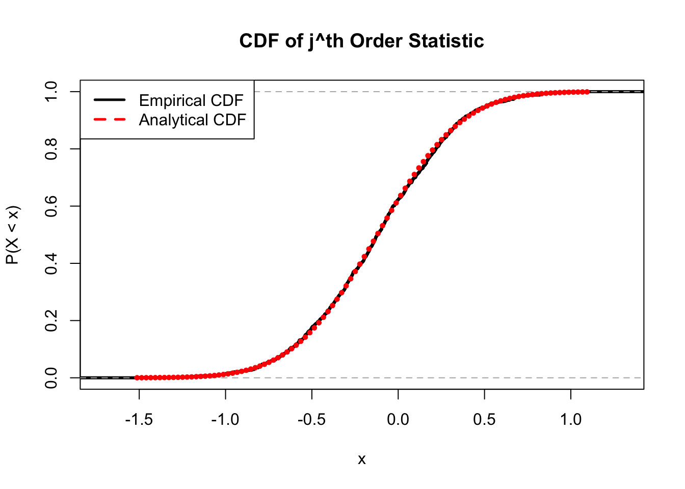

We’ve learned a lot about Order Statistics, but still haven’t seen why we decided to introduce this topic while learning about the Beta distribution. The reason is that there is a very interesting result regarding the Beta and the order statistics of Standard Uniform random variables.

Specifically, if we have that \(U_1, U_2,...,U_n\) are i.i.d. \(Unif(0, 1)\), then \(U_{(j)}\), the \(j^{th}\) order statistic, has a Beta distribution:

\[U_{(j)} = Beta(j, n - j + 1)\]

To prove this fact, we need to find the PDF of the \(j^{th}\) order statistic in general (much like how we found the CDF of the \(j^{th}\) order statistic above) which we won’t include here.

So, for example, if we have that \(U_1, U_2, U_3\) are i.i.d. \(Unif(0, 1)\), then the maximum of these random variables (i.e., \(U_{(3)}\), or the first order statistic) has a \(Beta(3, 1)\) distribution. This is an intuitive result because we know that the Uniform random variables marginally all have support from 0 to 1, so any order statistic of these random variables should also have support 0 to 1; of course, the Beta has support 0 to 1, so it satisfies this property. Additionally, consider if we have large \(j\) for the order statistic \(U_{(j)}\) (remember, this is the \(j^{th}\) smallest, so it will be a relatively large value). The distribution \(Beta(j, n - j + 1)\) will have a large first parameter \(j\) relative to the second parameter \(n - j + 1\) (since \(j\) is large). We know that the mean of a \(Beta(a, b)\) random variable is \(\frac{a}{a + b}\), so the mean in this case will be \(\frac{j}{n - j + 1 + j} = \frac{j}{n + 1}\), which is large when \(j\) is large. This makes sense: if \(j\) is large, then we are asking for the mean of one of the larger ranked random variables, which should intuitively have a high mean. The minimum random variable (or the first order statistic) has mean \(\frac{1}{n + 1}\), which is also intuitive: as \(n\) grows, this mean gets smaller and smaller (the more random variables we have, the closer to 0 we expect the minimum to be on average).

Recall that we said the Beta distribution was tricky because it didn’t have a conventional ‘story’ (i.e., the Exponential distribution measures time waited for a bus, etc.). Many statisticians consider this to be the story of a Beta distribution: the distribution of the order statistics of a Uniform. This result also helps to justify why we called the Beta a generalization of the Uniform earlier in this chapter!

We can check this interesting result with a simulation in R. We generate order statistics for a Uniform and check if the resulting distribution is Beta.

#replicate
set.seed(110)
sims = 1000

#define simple parameters
j = 7
n = 10


#keep track of Xj
Xj = rep(NA, sims)


#run the loop
for(i in 1:sims){
  
  #generate the data; use standard uniforms
  data = runif(n)
  
  #order the data
  data = sort(data)
  
  #find the j^th smallest
  Xj[i] = data[j]
}


#show that the j^th order statistic is Beta
#1x2 graphing grid
par(mfrow = c(1,2))

#Beta
hist(rbeta(sims, j, n + 1 - j), main = "Beta(j, n - j + 1)", 
     col = rgb(0, 0, 1, 1/4), xlab = "")

#Order Statistics
hist(Xj, main = "X_(j) for Unif(0, 1)",
     col = rgb(1, 0, 0, 1/4), xlab = "")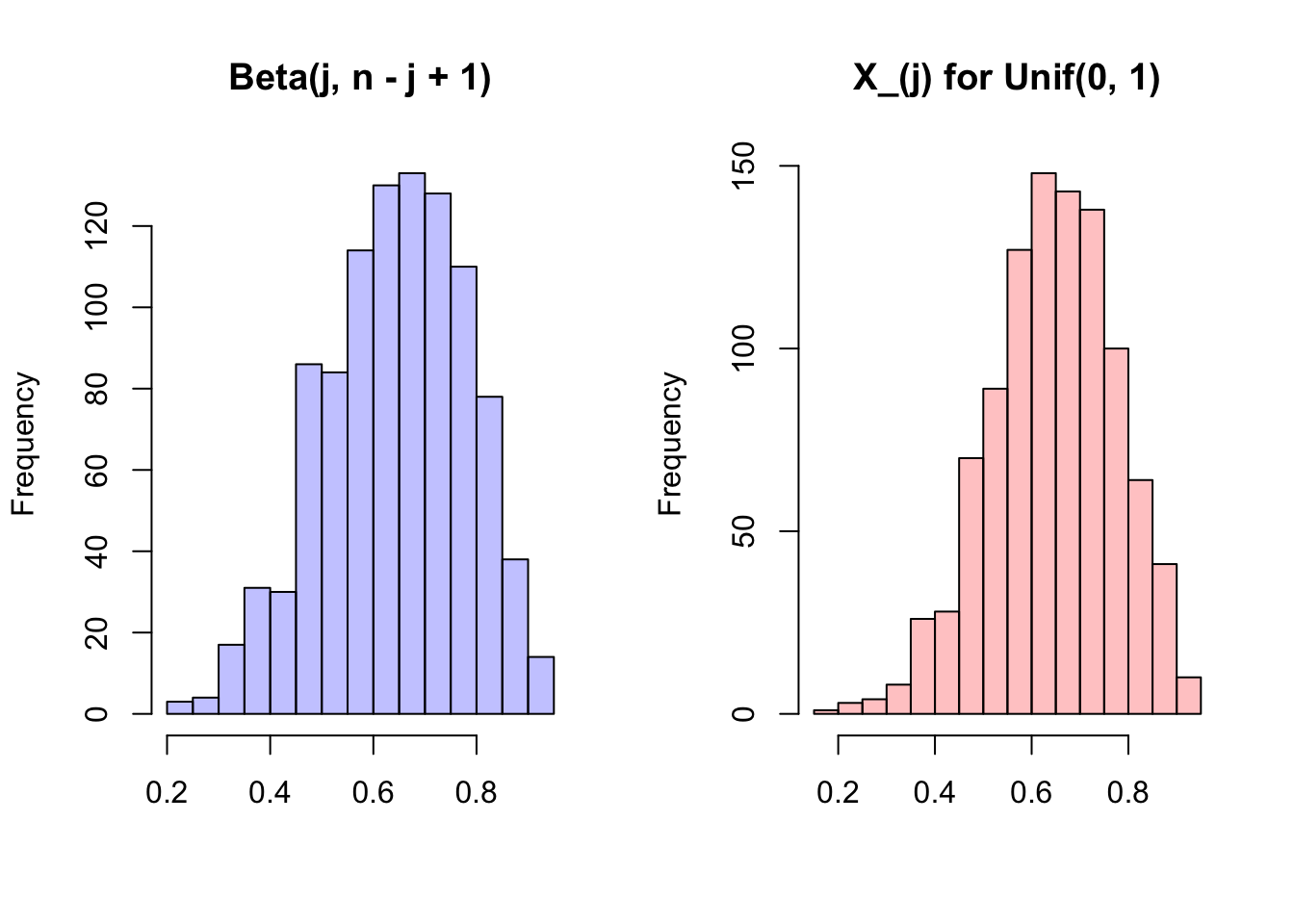

#re-set grid
par(mfrow = c(1,1))

Gamma

That’s about all we can do with the Beta (for now, at least), so we’ll move on to the second major distribution in this chapter: the Gamma distribution. Fortunately, unlike the Beta distribution, there is a specific story that allows us to sort of wrap our heads around what is going on with this distribution. It might not help with computation or the actual mechanics of the distribution, but it will at least ground the Gamma so that you can feel more comfortable with what you’re working with.

The Gamma has two parameters: if \(X\) follows a Gamma distribution, then \(X \sim Gamma(a, \lambda)\). Let’s jump right to the story. Recall the Exponential distribution: perhaps the best way to think about it is that it is a continuous random variable (it’s the continuous analog of the Geometric distribution) that can represent the waiting time of a bus. Also recall that the Exponential distribution is memoryless, so that it does not matter how long you have been waiting for the bus: the distribution going forward is always the same.

The Gamma distribution can be thought of as a sum of i.i.d. Exponential distributions (this is something we will prove later in this chapter). That is, if there are \(a\) buses, with each wait time independently distributed as \(Expo(\lambda)\), and you were interested in how long you would have to wait for the \(a^{th}\) bus, your wait time has the distribution \(Gamma(a,\lambda)\). Remember, this is a sum (the buses don’t arrive all at once, they come after each other, so after the \(j^{th}\) bus arrives we start the wait time for the \(j + 1^{th}\) bus), so we can formalize this distribution with notation: if we have \(Y = \sum_{j=1}^{a} X_j\) where each \(X_j\) is i.i.d. \(Expo(\lambda)\), then \(Y \sim Gamma(a, \lambda)\). What does this remind us of? Well, recall the Geometric distribution, which is the discrete companion of the Exponential, is just a simpler form of the Negative Binomial, which counts waiting time until the \(r^{th}\) success, not just the first success as the Geometric does. In that sense, the Gamma is similar to the Negative Binomial; it counts the waiting time for \(a\) Exponential random variables instead of the waiting time of \(r\) Geometric random variables (the sum of multiple waiting times instead of just one waiting time).

There’s a couple of ways to rigorously prove that a Gamma random variable is a sum of i.i.d. Exponential random variables; specifically, we know of two at the moment. We could either use a convolution (remember, convolutions give the distribution of sums) or MGFs (remember, the MGF of a sum is the product of individual MGFs). In this case, the latter is easier (we will explore this later in the chapter, after we learn a bit more about the Gamma).

So, that’s the story of a Gamma. Moving forward, we have that the expected value is \(\frac{a}{\lambda}\) and the variance is \(\frac{a}{\lambda^2}\) of a \(Gamma(a, \lambda)\) random variable. Of course, we could find these the usual way (with LoTUS, and we’ll see the PDF in a moment) or we could think about the connection to the Exponential, and the mean and variance of a single Exponential distribution. Remember that for \(X \sim Expo(\lambda)\), \(E(X) = \frac{1}{\lambda}\) and \(Var(X) = \frac{1}{\lambda^2}\). For the Gamma, based on the story we just learned, we are adding up \(a\) of these i.i.d. Exponential random variables. So, just imagine from the earlier example where \(T\) is the sum of \(a\) i.i.d. \(X \sim Expo(\lambda)\) random variables (so that every \(X\) has expectation \(\frac{1}{\lambda}\) and variance \(\frac{1}{\lambda^2}\)), and apply what we know about Expectation and Variance:

\[T = X_1 + X_2 + ... + X_a \rightarrow E(T) = E(X_1 + X_2 + ... + X_a) = E(X_1) + E(X_2) + ... + E(X_a) = \frac{a}{\lambda}\]

\[Var(T) = Var(X_1 + X_2 + ... + X_a) = Var(X_1) + Var(X_2) + ... + Var(X_a) = \frac{a}{\lambda^2}\]

And, thus, this is the mean and variance for a Gamma. Recall that, since we are taking a sum of Variances when we find \(Var(T)\), we also need all of the Covariances; however, since all \(X\)’s are i.i.d., every Covariance is 0 (independent random variables have Covariances of 0).

Now that we have a story for the Gamma Distribution, what is the PDF? Well, before we introduce the PDF of a Gamma Distribution, it’s best to introduce the Gamma function (we saw this earlier in the PDF of a Beta, but deferred the discussion to this point). This is marked in the field as \(\Gamma(a)\), and the definition is:

\[\Gamma(a) = \int_{0}^{\infty} x^{a-1}e^{-x}dx\]

Often, the \(x^{a-1}\) is written as \(x^a\) and you just divide by \(x\) elsewhere, but, if we write it in this way, all of the terms stay together.

This looks like a relatively strange function that doesn’t have a whole lot of application, but it’s actually quite useful and popular in mathematics because of its relationship to the factorial. Specifically, here are some interesting properties, for a positive integer \(n\):

\[\Gamma(n) = (n-1)!\] \[\Gamma(n+1) = n\Gamma(n)\]

You can probably see how these properties imply each other (since, using the first property, \(\Gamma(n + 1) = n! = n(n - 1)! = n\Gamma(n)\), which gives us the second property), and they allow us to find all sorts of values via the Gamma. So, really, \(\Gamma(5) = 4! = 24\). You could also say \(\Gamma(5) = 4\Gamma(4) = 4 \cdot 3!\), all the same thing. The key is not to be scared by this crane-shaped notation that shows up so often when we work with the Beta and Gamma distributions. This function is really just a different way to work with factorials.

Finally, let’s discuss the PDF. The PDF of a Gamma for \(X \sim Gamma(a,1)\) (just let \(\lambda = 1\) now for simplicity) is:

\[f(x) = \frac{1}{\Gamma(a)} x^{a-1} e^{-x}\]

How did we get to this result? We wanted to create a PDF out of the Gamma function, \(\Gamma(a)\). We know, of course, that the PDF must integrate to 1 over the support, which in this case is all positive numbers (note that this is also the support of an Exponential, and it makes sense here, since we’re just waiting for multiple buses instead of one). So, what we’re going to do is take the equation for the Gamma function and simply divide both sides by \(\Gamma(a)\):

\[\Gamma(a) = \int_{0}^{\infty} x^{a-1}e^{-x}dx \longrightarrow 1 = \int_{0}^{\infty}\frac{1}{\Gamma(a)} x^{a-1}e^{-x}dx\]

So, since we know that the RHS of the equation on the right, \(\frac{1}{\Gamma(a)} x^{a-1}e^{-x}\), integrates to 1, we allow it to be our PDF (we’ll see more of this type of reasoning later in the chapter when we discuss Pattern Integration). It seems kind of crude, but this is the idea behind forging the PDF of a Gamma distribution (and the reason why it is called the Gamma!)

However, this is of course just in the simple case when \(\lambda = 1\), and we want to find the PDF in a more general case where we just have general \(\lambda\). That is, if we let \(X \sim Gamma(a, 1)\) and \(Y \sim Gamma(a, \lambda)\), we want to calculate the PDF of \(Y\). We know that, by the transformation theorem that we learned back in Chapter 7:

\[f(y) = f(x) \frac{dx}{dy}\]

First, then, we need to solve for \(X\) in terms of \(Y\). Recall an interesting fact of the Exponential distribution, which we referred to as a ‘scaled Exponential’: if \(Z \sim Expo(\lambda)\), then \(\lambda Z \sim Expo(1)\). We can actually apply this here: we can say that \(X = \lambda Y\), even though \(X\) and \(Y\) are Gamma and not Exponential. Why can we so quickly say that this is true? Well, the Gamma distribution is just the sum of i.i.d. \(Expo(\lambda)\) (and, specifically, we have \(a\) of them), so when we multiply a Gamma random variable by \(\lambda\), we are essentially multiplying each \(Expo(\lambda)\) random variable by \(\lambda\). We know from the ‘scaled Exponential’ result that a \(Expo(\lambda)\) random variable multiplied by \(\lambda\) is just an \(Expo(1)\) random variable, and we are then adding \(a\) of these random variables, so we are left with a \(Gamma(a, 1)\) random variable. We can now write out the RHS of the transformation theorem above, plugging in the PDF of \(X\) and \(\frac{dx}{dy}\). We just showed that \(X = \lambda Y\), so \(\frac{dx}{dy}\), or the derivative of \(X\) in terms of \(Y\), is just \(\lambda\) (since \(\lambda Y\) is equal to \(X\), and we just derive this in terms of \(Y\)).

\[f(y) = \frac{1}{\Gamma(a)} x^{a - 1} e^{-x} \lambda\]

We now plug in \(\lambda y\) every time we see an \(x\):

\[ = \frac{1}{\Gamma(a)} (\lambda y)^{a - 1} e^{-\lambda y} \lambda\] \[ = \frac{\lambda^a}{\Gamma(a)} y^{a - 1} e^{-\lambda y} \]

So, this is our PDF for the general case \(Y \sim Gamma(a,\lambda)\).

Remember, this random variable is just the sum of \(a\) independent Exponential random variables, each with parameter \(\lambda\). In fact, let’s do a quick sanity check to make sure that this PDF is valid. If \(a=1\), we’re essentially working with just one Exponential random variable, so \(Gamma(1,\lambda)\) should have the same distribution as \(Expo(\lambda)\). If we plug in \(a=1\) to the PDF of a Gamma, then, this should collapse to an Exponential PDF. Let’s see: we know that \(\Gamma(1) = (1-1)! = 0! = 1\), and \(y^{1 - 1} = y^0 = 1\), and we are then left with \(\lambda e^{-\lambda y}\), which is indeed the PDF of an \(Expo(\lambda)\) random variable. So, our sanity check works out.

You can further familiarize yourself with the Gamma distribution with this Shiny App; reference this tutorial video for more.

Click here to watch this video in your browser. As always, you can download the code for these applications here.

Beta and Gamma

Hopefully these distributions did not provide too steep a learning curve; understandably, they can seem pretty complicated, at least because they seem so much more vague than the distributions we have looked at thus far (especially the Beta) and their PDFs involve the Gamma function and complicated, un-intuitive constants. They are probably the two hardest distributions we’ve dealt with so far. We will now discuss their relationship to each other, which is also very important (recall that connections between random variables are often more interesting than the random variables marginally).

We’ve already done most of the heavy lifting for each of these distributions, so we can now feel comfortable discussing their relationship. Specifically, Professor Blitzstein calls this the “Bank-Post Office” Problem and, similar to the “Chicken and Egg” Problem, it helps to reveal some really interesting results with the involved distributions.

The set-up is as follows: you have two different errands to run, one at the Bank and one at the Post Office. Both places are notorious for having lines that you have to wait in before you actually reach the counter. Let the time you wait at the Bank be distributed \(X \sim Gamma(a, \lambda)\) and the time you wait at the Post Office be distributed \(Y \sim Gamma(b,\lambda)\). These wait times are independent.

Now let’s consider your total wait time, \(T\), such that \(T = X + Y\), and the fraction of the time you wait at the Bank, \(W\), such that \(W = \frac{X}{X+Y}\). The problem is to find the joint distribution of \(T\) and \(W\).

This is an excellent problem to help us practice our work with transformations, as well as the Beta and Gamma distributions. Recall that we learned about 2-D transformations in Chapter 7, but we didn’t actually do an example; now, then, is our first chance to implement what we have learned. Recall the formula for a 2-D transformation:

\[f(t, w) = f(x, y) \left( \begin{array}{cc} \frac{\partial x}{\partial t} & \frac{\partial x}{\partial w} \\ \frac{\partial y}{\partial t} & \frac{\partial y}{\partial w}\end{array} \right)\]

In words, this is saying that the joint PDF of \(T\) and \(W\), \(f(t, w)\), is equal to the joint PDF of \(X\) and \(Y\), \(f(x, y)\) (with \(t\) and \(w\) plugged in for \(x\) and \(y\)) times this Jacobian matrix.

Let’s walk through each piece. First, \(f(x, y)\) should be easy: since we are given that \(X\) and \(Y\) are independent, we know that \(f(x, y) = f(x) f(y)\) (recall, similar to probabilities, we can multiply marginal distributions to get joint distributions in the independent case). Both \(X\) and \(Y\) are Gamma random variables, so we know their PDFs. We can start to plug in:

\[f(t, w) = \frac{\lambda^a}{\Gamma(a)} \cdot x^{a - 1} \cdot e^{-\lambda x} \cdot \frac{\lambda^b}{\Gamma(b)} \cdot y^{b - 1} \cdot e^{-\lambda y} \left( \begin{array}{cc} \frac{\partial x}{\partial t} & \frac{\partial x}{\partial w} \\ \frac{\partial y}{\partial t} & \frac{\partial y}{\partial w}\end{array} \right)\]

Next, we should plug in \(t\) and \(w\) terms wherever we see \(x\) and \(y\). First, this means that we have to solve for \(x\) and \(y\) in terms of \(t\) and \(w\). We know that \(t = x + y\), and then we know \(w = \frac{x}{x + y}\), so we can plug in \(t\) for \(x + y\) to get \(w = \frac{x}{t}\). Solving this yields \(x = wt\). It’s then easy to plug in \(wt\) for \(x\) in \(t = x + y\), and solving yields \(t(1 - w) = y\). Now, we just have to plug in \(tw\) every time we see \(x\) in the above equation, and \(t(1 - w)\) every time we see \(y\).

\[f(t, w) = \frac{\lambda^a}{\Gamma(a)} \cdot (tw)^{a - 1} \cdot e^{-\lambda tw} \cdot \frac{\lambda^b}{\Gamma(b)} \cdot (t(1 - w))^{b - 1} \cdot e^{-\lambda t(1 - w)} \left( \begin{array}{cc} \frac{\partial x}{\partial t} & \frac{\partial x}{\partial w} \\ \frac{\partial y}{\partial t} & \frac{\partial y}{\partial w}\end{array} \right)\]

Let’s now focus on the Jacobian. The top left entry is the derivative of \(x\) in terms of \(t\), the top right entry is the derivative of \(x\) in terms of \(w\), etc. Since we know \(x = tw\) and \(y = t(1 - w)\), these derivatives are easy (for example, to find the derivative of \(x\) in terms of \(t\), we realize that \(tw = x\), so we just derive \(tw\) in terms of \(t\) to get \(w\)). Completing these derivatives yields:

\[f(t, w) = \frac{\lambda^a}{\Gamma(a)} \cdot (tw)^{a - 1} \cdot e^{-\lambda tw} \cdot \frac{\lambda^b}{\Gamma(b)} \cdot (t(1 - w))^{b - 1} \cdot e^{-\lambda t(1 - w)} \left( \begin{array}{cc} w & t\\ 1 - w & -t \end{array} \right)\]

We now just have to calculate the absolute determinant of this Jacobian matrix, which is just \(|ab - cd|\), if \(a\) is the top left entry, \(b\) is the top right entry, etc. This yields:

\[|-wt - t(1 - w)| = |-wt - t + tw| = t\]

So, this entire term just simplifies to \(t\). We are left with:

\[f(t, w) = \frac{\lambda^a}{\Gamma(a)} \cdot (tw)^{a - 1} \cdot e^{-\lambda tw} \cdot \frac{\lambda^b}{\Gamma(b)} \cdot (t(1 - w))^{b - 1} \cdot e^{-\lambda t(1 - w)} t\]

We can combine terms to make this look a lot nicer:

\[f(t, w) = \frac{\lambda^{a + b}}{\Gamma(a + b)}t^{a + b - 1}e^{-\lambda t} w^{a - 1} (1 - w)^{b - 1}\]

This looks better! Now, let’s take a second and think about the distribution of \(T\). We know that \(T = X + Y\), where \(X\) and \(Y\) are i.i.d. Gamma random variables; specifically, \(X \sim Gamma(a, \lambda)\) and \(Y \sim Gamma(b, \lambda)\). Consider the story of a \(Gamma(a, \lambda)\) random variable: it is the sum of i.i.d. \(Expo(\lambda)\) random variables. Therefore, the sum of two independent Gamma random variables (both with rate parameter \(\lambda\)) is just one massive sum of i.i.d. \(Expo(\lambda)\) random variables! How many of these random variables do we have? Simply \(a + b\) of them, and then we are left with another Gamma random variable! That is, \(T \sim Gamma(a + b, \lambda)\).

So, we actually know what the distribution of \(T\) is, and this can help us deal with our joint PDF. That is, we should look for the PDF of \(T\), which we know to be \(\frac{\lambda^{a + b}}{\Gamma(a + b)}t^{a + b - 1}e^{-\lambda t}\), in our joint PDF. We actually almost have this; if we group terms, we see:

\[f(t, w) = \Big(\lambda^{a + b} t^{a + b - 1}e^{-\lambda t}\Big) \Big(\frac{1}{\Gamma(a + b)}w^{a - 1} (1 - w)^{b - 1}\Big)\]

The term on the left is very close to \(\frac{\lambda^{a + b}}{\Gamma(a + b)}t^{a + b - 1}e^{-\lambda t}\), the correct PDF of \(T\): it’s simply missing a \(\frac{1}{\Gamma(a + b)}\) term. We can fix this; we just multiply and divide by this term (we’ll get more used to this type of approach when we do ‘Pattern Integration’ later in this chapter):

\[f(t, w) = \Big(\frac{\lambda^{a + b}}{\Gamma(a + b)} t^{a + b - 1}e^{-\lambda t}\Big) \Big(\frac{\Gamma(a + b)}{\Gamma(a + b)}w^{a - 1} (1 - w)^{b - 1}\Big)\]

There! The term on the left is now the full PDF of a \(Gamma(a + b, \lambda)\) random variable.

Have you been paying attention to the term on the right? This is the PDF of \(W\) (we know it is the PDF of \(W\) because everything else is the PDF of \(T\)); Does it look like a PDF that we know? At this point, we have actually reached a couple of really interesting results.

1. \(T \sim Gamma (a+b,1)\) and \(W \sim Beta(a,b)\) (we know the distribution of \(W\) because the term on the right, or the PDF of \(W\), is the PDF of a \(Beta(a, b)\)). Again, you didn’t have to do this laborious calculation to find the distribution \(T\), since we are summing independent and identical Exponential distributions (all have rate parameter \(\lambda\)) which we know becomes a Gamma (wait time for multiple buses is Gamma). However, the result for \(W\) is interesting and important; it is interesting that this fraction of Gammas turns out to be Beta! The support, at least, makes sense, since \(\frac{X}{X + Y}\) is bounded between 0 and 1, like a Beta random variable.

2. \(T\) and \(W\) are independent because we can factor the joint PDF into the two marginal PDFs; in practical terms, the total wait time is independent of the fraction of time that we wait at the Bank. We know this because the joint PDF that we see above is just the product of the marginal PDFs of the \(Gamma(a + b, 1)\) random variable and the \(Beta(a, b)\) random variable. An interesting fact is that the Gamma distribution is the only distribution that allows for this independence result (starting with \(X\) and \(Y\) as Gamma random variables, that is; \(X\) and \(Y\) couldn’t be any other distributions if we want \(T\) and \(W\) to be independent). This is not super intuitive (not immediately obvious that the total wait time and the fraction of wait time at one place are independent) and it’s similar to the Chicken and Egg result that claimed the number of eggs was independent from the number that hatched (although this Bank-Post Office result is probably a little less surprising).

3. This process serves as a sort of proof for normalizing constant for a \(Beta(a,b)\) random variable: \(\frac{\Gamma(a+b)}{\Gamma(a)\Gamma(b)}\). That is, we know the term on the right is a PDF of a \(Beta(a, b)\), since we have \(w^{a - 1}(1 - w)^{b - 1}\) (and we have no more \(w\) terms in the rest of the term), so the constant that is left over must be the valid normalizing constant (if we did all of our calculations correctly).

We can confirm our results in R by simulating from the relevant distributions. We’ll take many draws for \(X\) and \(Y\) and use these to calculate \(T\) and \(W\). Then, we’ll see if \(T\) and \(W\) take on the distributions that we solved for. We’ll also see if the mean of \(T\) changes if we condition on specific values for \(W\). We found that the two are independent, so the mean should not change; of course, this single point check doesn’t rigorously prove independence, but it is reassuring that the mean doesn’t change!

#replicate
set.seed(110)
sims = 1000

#define simple parameters
lambda = 5
a = 3
b = 4

#generate the r.v.'s
X = rgamma(sims, a, lambda)
Y = rgamma(sims, b, lambda)

#combine the r.v.'s; use Z instead of T, since T is saved as TRUE in R
Z = X + Y
W = X/(X + Y)

#set a 2x2 graphing grid
par(mfrow = c(2,2))

#plots should match the respective distributions
hist(Z, main = "T", col = rgb(1,0,0,1/4), xlab = "")
hist(rgamma(sims, a + b, lambda), main = "Gamma(a + b, lambda)", col = rgb(1,0,0,1/4), xlab = "")
hist(W, main = "W", col = rgb(0,1,0,1/4), xlab = "")
hist(rbeta(sims, a, b), main = "Beta(a, b)", col = rgb(0,1,0,1/4), xlab = "")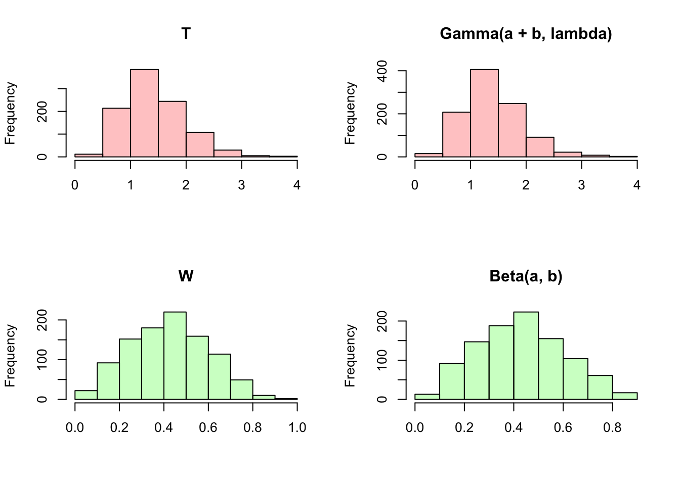

#re-set grid
par(mfrow = c(1,1))

#mean does not change
mean(Z)

## [1] 1.415373

mean(Z[W > 1/2])

## [1] 1.404945

So, it’s clear that these two intense distributions are interwoven in deep and complex ways. Again, the most important thing to take away from Bank-Post Office is strictly the result, which is listed out above. It is good practice to solve this problem, though, especially to get experience with multi-dimensional transformation (we get to work through and find the Joint PDF of \(W\) and \(T\)).

Pattern Integration

When you first took calculus, you probably learned a variety of different integration methods: u-substitution, integration by parts, etc. In this section, we’re going to discuss a new method of integration directly related to our work in this book. This is not a calculus book, and while we are performing calculus calculations, we’ll see how these problems are still centered around probability.

It’s probably best to start with an example. Imagine that you were asked to calculate the following integral:

\[\int_{0}^1 x^{a - 1}(1 - x)^{b - 1} dx\]

Where \(a\) and \(b\) are constants (notice the \(dx\); this means, of course, that we are integrating with respect to \(x\)). This does not look like a trivial integral to solve. We could try integrating by parts or by making a substitution, but none of these strategies seem to be immediately promising (although they do seem to ‘promise’ a lot of work!).

Instead, and you likely may have guessed this by now, we can work to recognize that this integrand is related to something we know intimately (the ‘pattern’ in ‘pattern integration’). Specifically, recall the Beta PDF from earlier in the chapter. If \(X \sim Beta(a, b)\), then:

\[f(x) = \frac{\Gamma(a + b)}{\Gamma(a) \Gamma(b)} x^{a - 1}(1 - x){b - 1}\]

Also recall that we called \(\frac{\Gamma(a + b)}{\Gamma(a) \Gamma(b)}\) the normalizing constant, because it is a constant value (not a function of \(x\), so not changing with \(x\)) that allows the PDF to integrate to 1. If this is called the normalizing constant, then, we will call \(x^{a - 1}(1 - x)^{b - 1}\) the ‘meaty’ part of the PDF. The label ‘meaty’ is appropriate because it’s the ‘important’ part of the PDF: the part that changes with \(x\), which is the random variable that we actually care about!

So, we can recognize that the integral we need to find, \(\int_{0}^1 x^{a - 1}(1 - x)^{b - 1} dx\), is the ‘meaty’ part of a \(Beta(a, b)\) PDF. Now that we have recognized what PDF this is similar to, we can use the fact that valid PDFs, when integrated over their support, must integrate to 1. Here, we are integrating from 0 to 1, which we know to be the support of a Beta. Therefore (and this is the big step) we multiply and divide by the normalizing constant:

\[\int_{0}^1 x^{a - 1}(1 - x)^{b - 1} dx\] \[=\frac{\Gamma(a)\Gamma(b)}{\Gamma(a + b)}\int_{0}^1\frac{\Gamma(a + b)}{\Gamma(a) \Gamma(b)} x^{a - 1}(1 - x)^{b - 1} dx \]

That is, we multiplied by \(\frac{\Gamma(a + b)}{\Gamma(a) \Gamma(b)}\) and divided by the reciprocal \(\frac{\Gamma(a)\Gamma(b)}{\Gamma(a + b)}\), so that we didn’t change the equation (essentially, we are multiplying by 1; imagine multiplying by 2 and then dividing by 2, the equation stays unchanged; we can put one outside of the integral and one inside of the integral because they are both constants in that they don’t change with respect to \(x\), the variable of integration). Why would we do this unnecessary multiplication and division if it doesn’t change the value of the equation? Well, notice that we now have \(\int_{0}^1\frac{\Gamma(a + b)}{\Gamma(a) \Gamma(b)} x^{a - 1}(1 - x)^{b - 1} dx\), which we know to be the PDF of a \(Beta(a, b)\) random variable integrated over its support (0 to 1), meaning that it must integrate to 1. We are thus left with an elegant result:

\[=\frac{\Gamma(a)\Gamma(b)}{\Gamma(a + b)}\]

We can confirm that this is the correct result in R. We will define a function for the integrand, and then use the integrate function in R to complete the integration over a specified bound.

#define simple parameters
a = 3
b = 2

#define a function for the integrand
integrand = function(x){
  return(x^(a - 1)*(1 - x)^(b - 1))
}

#these should match
integrate(integrand, 0, 1); (gamma(a)*gamma(b))/gamma(a + b)

## 0.08333333 with absolute error < 9.3e-16

## [1] 0.08333333

This is pretty interesting way to think about solving integrals. We essentially did no actual calculus, yet were able to complete this difficult integral using our knowledge of probability distributions. We recognized that we were close to a valid PDF, ‘completed’ the PDF, and used the fact that valid PDFs must integrate to 1. This problem (and pattern integration in general) is an excellent example of how taking time to think about a problem can result in a much more simple, elegant solution than the straightforward, brute force calculation would provide. We’ll consider one more example to make sure that we really understand what’s going on.

Example 8.1

Calculate the integral:

\[\int_{0}^{\infty} \sqrt{x} \; e^{-x}dx\]

This looks like a prime candidate for integration by parts; however, we don’t want to do integration by parts; not only is this not a calculus book, but it is a lot of work! Instead, does this integrand look similar to a PDF that we are familiar with? Recall the PDF of a Gamma random variable. If \(Y \sim Gamma(a, \lambda)\), then:

\[f(y) = \frac{\lambda^a}{\Gamma(a)} y^{a - 1} e^{-\lambda y} \]

Now, imagine writing out the PDF for a \(Gamma(3/2, 1)\) random variable. If \(X \sim Gamma(3/2, 1)\), then:

\[f(x) = \frac{1}{\Gamma(3/2)} y^{3/2 - 1} e^{-y}\] \[ = \frac{1}{\Gamma(3/2)} \sqrt{y} \; e^{-y}\]

Now, we can see that the integral we were asked to calculate, \(\int_{-\infty}^{\infty} \sqrt{x} \; e^{-x}dx\), looks a lot like the ‘meaty’ part of a \(Gamma(3/2, 1)\) random variable. We multiply and divide by the normalizing constant \(\frac{1}{\Gamma(3/2)}\):

\[\int_{0}^{\infty} \sqrt{x} \; e^{-x}dx\] \[= \Gamma(3/2) \int_{0}^{\infty} \frac{1}{\Gamma(3/2)}\sqrt{x} \; e^{-x}dx\]

And, now, the integrand is the PDF of a \(Gamma(3/2, 1)\) random variable, integrated over the support (recall the story of the Gamma: waiting time for multiple buses, so the support is all positive numbers). Therefore, we know that the PDF integrates to 1, and we are left with:

\[= \Gamma(3/2)\]

Again, a simple result for a complicated integral!

We can again confirm this result in R. As above, we define a function for the integrand, and then use the integrate function to integrate this function over the support. This should match our analytical result of \(\Gamma(3/2)\), which we solved above.

#define a function for the integrand
integrand = function(x){
  return(sqrt(x)*exp(-x))
}

#these should match (remember, infinity is stored as Inf in R)
integrate(integrand, 0, Inf); gamma(3/2)

## 0.8862265 with absolute error < 2.5e-06

## [1] 0.8862269

Example 8.2 (Story of the Gamma)

Earlier in this chapter, we defined the story of a \(Gamma(a, \lambda)\) random variable as the sum of \(a\) i.i.d. \(Expo(\lambda)\) random variables. However, we didn’t prove this fact. Now, let’s give a proof that shows this fact to be true. In the past, how have we shown that two distributions are the same? One common way is via the MGF (if two random variables have the same MGF, then they must have the same distribution).

Here, we can try to show that the MGF of the sum of \(a\) i.i.d. \(Expo(\lambda)\) random variables is the same as the MGF of a \(Gamma(a, \lambda)\) random variable. We can also use the fact that the MGF of a sum of random variables is equal to the product of the MGFs of the individual random variables. Recall our calculation for the MGF of \(X \sim Expo(\lambda)\) from Chapter 5:

\[M(t) = \int_{0}^{\infty} e^{tx}\lambda e^{-x\lambda} dx = \lambda\int_{0}^{\infty} e^{-x(\lambda-t)} = -\lambda \frac{e^{-x(\lambda-t)}}{\lambda-t}\Big|_{0}^{\infty} = \frac{\lambda}{\lambda-t}\] So, by the multiplicative property of MGFs (the MGF of a sum is the product of the individual MGFs) we know that the MGF of the sum of \(a\) i.i.d. \(Expo(\lambda)\) random variables is \(\Big(\frac{\lambda}{\lambda - t}\Big)^a\). We thus have to see if the MGF of a \(Gamma(a, \lambda)\) random variable equals this value.

Let’s try to complete the calculation! Letting \(X \sim Gamma(a, \lambda)\), and knowing the definition of the MGF is \(E(e^{tX})\) (as well as the PDF of \(X\)), we set up the LOTUS calculation:

\[E(e^{tX}) = \int_0^{\infty} e^{tx} \frac{\lambda^a}{\Gamma(a)} x^{a - 1} e^{-\lambda x}dx\] Factoring out the constants, and combining terms in the exponent:

\[= \frac{\lambda^a}{\Gamma(a)}\int_0^{\infty} x^{a - 1} e^{x(t -\lambda)}dx\]

This looks like a difficult integral, but recall the ‘Pattern Integration’ techniques we’ve just learned. In fact, we can notice that \(x^{a - 1} e^{x(t -\lambda)}\) looks like the ‘meaty’ part (where ‘meaty’ is defined above) of a \(Gamma(a, \lambda - t)\) (be careful, it’s not \(t - \lambda\); don’t forget the negative sign in the exponent!). Therefore, we can multiply by the normalizing constant (and the reciprocal of the normalizing constant) to get:

\[= \frac{\lambda^a}{\Gamma(a)} \cdot \frac{\Gamma(a)}{(\lambda - t)^a}\int_0^{\infty} \frac{(\lambda - t)^a}{\Gamma(a)} x^{a - 1} e^{x(t -\lambda)}dx\]

And now we know that the integrand is just the PDF of a \(Gamma(a, \lambda - t)\) random variable, so it goes to 1. We are left with:

\[=\frac{\lambda^a}{\Gamma(a)} \cdot \frac{\Gamma(a)}{(\lambda - t)^a}\] \[= \frac{\lambda^a}{(\lambda - t)^a}\] \[\Big(\frac{\lambda}{\lambda - t}\Big)^a\]

Which is, in fact, equal to the MGF of the sum of \(a\) i.i.d. \(Expo(\lambda)\) random variables! Therefore, since these have the same MGF, they have the same distribution, which was what we were trying to prove (and were able to prove using Pattern Integration!).

We can confirm this fact in R by generating random variables using rgamma and rexp.

#replicate
set.seed(110)
sims = 1000

#define simple parameters
a = 10
lambda = 5

#generate from the Gamma
gammas = rgamma(sims, a, lambda)

#generate from the Expos; bind into a matrix and calculate sums
expos = rexp(sims*a, lambda)
expos = matrix(expos, nrow = sims, ncol = a)
expos = rowSums(expos)

#set 2x1 graphing grid
par(mfrow = c(1,2))

#histograms should match
hist(gammas, main = "Gamma(a, lambda)", col = rgb(0, 0, 1, 1/4), xlab = "")
hist(expos, main = "Sum of i.i.d. Expo(lambda) r.v.s", col = rgb(0, 1, 0, 1/4), xlab = "")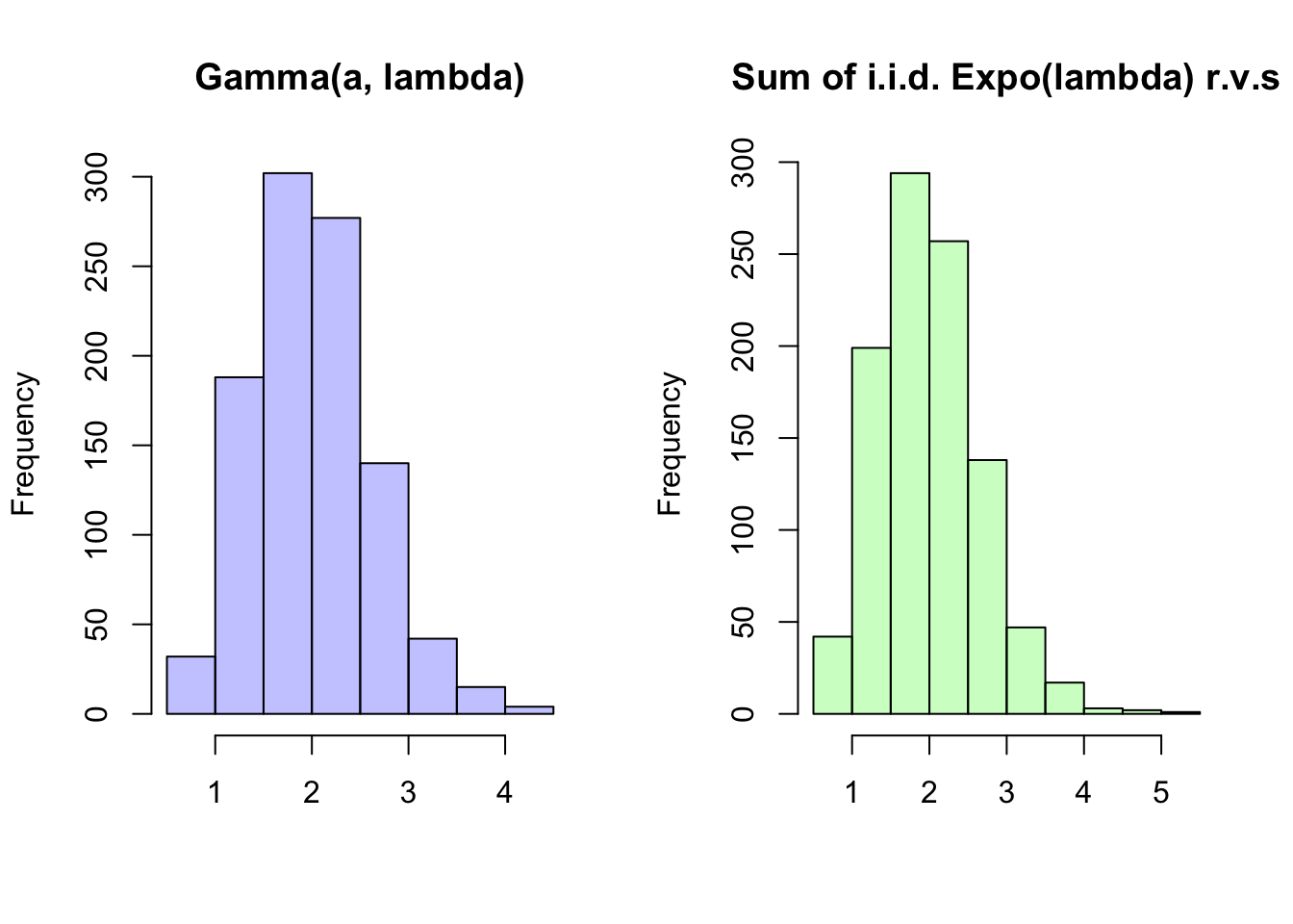

#re-set graphing grid
par(mfrow = c(1,1))

We can consider one more example of Pattern Integration with the video below. In this video, we calculate the variance of a Beta random variable.

Click here to watch this video in your browser.

Poisson Process

Before we close with this chapter, we’ll talk about one more interesting connection between two distributions that we are already familiar with. Remember, the relationship between different distributions is very important in probability theory (in this chapter alone, we saw how the Beta and Gamma are linked). Now, we’ll connect the Poisson and the Exponential.

This is a pretty interesting bridge, because we are crossing from a discrete distribution (Poisson) to a continuous one (Exponential). The classic example is to imagine receiving emails in an inbox. However, we’ll modernize it to receiving texts on a phone. Consider one interval, perhaps from time 0 to time \(t\). Assume that the number of texts received in disjoint time intervals (i.e., non-overlapping intervals like \([0, 4]\) and \([7.5, 9]\)) are independent.

Now say that the waiting time until a text arrives is distributed \(Expo(\lambda)\). Remember, the Exponential distribution is memoryless, so we don’t have to worry about where we are on the interval (i.e., how long we’ve already waited). Also assume that as soon as a text arrives, we start waiting for another one (and, of course, this wait time is also independently distributed \(Expo(\lambda)\); we can also think of this as the ‘time between arrivals’). If indeed this is true (the time between arrivals is an \(Expo(\lambda)\) random variable), then the total number of texts received in that time interval from 0 to \(t\), which we will call \(N\), is distributed \(N \sim Pois(\lambda t)\). We call \(N\) a ‘Poisson process with rate parameter \(\lambda\).’

We won’t engage too deeply with this result (there are many interesting branches and applications, but they are more appropriately reserved for a Stochastic Processes course), but let’s think about why it makes sense. The Exponential distribution models the wait time for some event, and here we are modeling the wait time between texts, so this structure makes sense. The Poisson distribution models the number of occurrences of a ‘rare’ or ‘unlikely’ event, and here we are using the Poisson to do just that (there are many individual ‘time-stamps’ in this interval, and a small chance that any one specific time-stamp has a text arriving). Even the set-up makes sense: the parameter \(\lambda\) for the Exponential is essentially a rate parameter, and ultimately gives the amount of events you should expect in one unit of time (remember that the mean of an Exponential is \(\frac{1}{\lambda}\), which means the average wait time decreases as you expect more events - quantified by the rate parameter \(\lambda\) - increases). So, when we want to measure how many actual events there are instead of just measuring the time in between them, it makes sense to multiply \(\lambda\), the rate, by the length of the interval, \(t\). We can consider a simple example to fully solidify this concept of Poisson Processes; here, we will present both analytical and empirical solutions.

Example 8.3 (Facebook)

Let the number of Facebook notifications that you receive in a 2 hour interval be a Poisson Process with rate parameter \(\lambda\) (where \(\lambda\), a known constant, is given as an hourly rate; i.e., number of notifications received per hour).

1. How many notifications do we expect in this 2 hour interval?

Analytical Solution:

Let \(X\) be the number of notifications we receive in this interval. If we are concerned with a 2 hour interval, then \(X \sim Pois(2 \lambda)\), by the story of a Poisson Process (multiply the length of the interval by the rate parameter to get the parameter of the Poisson). Therefore, we expect \(2\lambda\) notifications in this interval, which makes sense, since we expect \(\lambda\) notifications every hour!

Empirical Solution:

#replicate
set.seed(110)
sims = 1000

#define a simple parameter
lambda = 1

#count how many notifications we get
notifications = rep(0, sims)

#run the loop
for(i in 1:sims){
  
  #keep track of the time; initialize here
  time = 0
  
  #go for two hours
  while(TRUE){
    
    #add an arrival
    time = time + rexp(1, lambda)
    
    #see if we're past two hours; break if we are
    if(time > 2){
      break
    }
    
    #otherwise, count the notification (arrived within 2 hours)
    notifications[i] = notifications[i] + 1
  }
}

#should get 2*lambda = 2
mean(notifications)

## [1] 2.041

2. In the first 90 minutes, we get 0 notifications. What is the probability that we get a notification in the next 30 minutes?

Analytical Solution:

We know that arrivals in disjoint intervals for a Poisson process are independent. Additionally, \(\lambda\) is known (as given in the prompt); if it wasn’t known, then observing 0 notifications in the first 90 minutes would give us information about an unknown \(\lambda\) (i.e., we expect \(\lambda\) to be near 0). However, in this case, this final 30 minutes is independent of the first 90 minutes. Again, then, let \(X\) be the number of notifications we receive in this interval. By the story of a Poisson Process, then, \(X \sim Pois(\lambda/2)\) (since the interval we are considering now is \(1/2\) hours long, and \(\lambda\) is still our rate parameter). So, we need the probability that \(X > 0\). We write:

\[P(X > 0) = 1 - P(X = 0) = 1 - e^{\lambda/2}\]

Further, we could think of this problem in terms of an Exponential random variable; we know that wait times are distributed \(Expo(\lambda)\), so we just need the probability that this wait time (i.e., the wait time for the next notification) doesn’t exceed 1/2 (we say 1/2 instead of 30 minutes because we are working in hour units, not minutes). This is just \(P(Y \leq 1/2)\) if \(Y \sim Expo(\lambda)\), and, given the CDF of an Exponential random variable (which you can always look up if you forget it, or re-derive by integrating the PDF) we write:

\[P(Y \leq 1/2) = 1 - e^{-\lambda/2}\]

Which of course matches the solution we got by taking a Poisson approach.

Empirical Solution:

#replicate
set.seed(110)
sims = 1000

#define a simple parameter
lambda = 1

#indicators if we get 0 notifications in first 90 minutes, and
#   at least one notification in last 30 minutes
first.90 = rep(1, sims)
last.30 = rep(0, sims)

#run the loop
for(i in 1:sims){
  
  #keep track of the time; initialize here
  time = 0
  
  #go for two hours
  while(TRUE){
    
    #add an arrival
    time = time + rexp(1, lambda)
    
    #see if we're past two hours; break if we are
    if(time > 2){
      break
    }
    
    #if we get an arrival in first 90 minutes, first indicator didn't occur
    if(time < 3/2){
      first.90[i] = 0
    }
    
    #mark if the arrival is in the last half hour
    if(time > 3/2){
      last.30[i] = 1
    }
  }
}

#should get 1 - exp(-lambda/2) = .393
mean(last.30[first.90 == 1])

## [1] 0.3911111

#should also match the unconditional case
mean(last.30)

## [1] 0.381

3. Let \(Y\) be the wait time until we have received 5 notifications. Find \(E(Y)\) and \(Var(Y)\).

Analytical Solution:

We know that wait time between notifications is distributed \(Expo(\lambda)\), and essentially here we are considering 5 wait times (wait for the first arrival, then the second, etc.). So, we can think of \(Y\) as the sum of 5 i.i.d. \(Expo(\lambda)\) random variables. We learned in this chapter that this has a \(Gamma(5, \lambda)\) distribution, by the story of the Gamma distribution (sum of i.i.d. Exponential random variables), so we can easily look up the expectation and variance of \(Y\):

\[E(Y) = \frac{5}{\lambda}, \; Var(Y) = \frac{5}{\lambda^2}\]

Empirical Solution:

#replicate
set.seed(110)
sims = 1000

#define a simple parameter
lambda = 1

#keep track of the final time
time = rep(0, sims)

#run the loop
for(i in 1:sims){
  
  #generate 5 arrivals
  for(j in 1:5){
    
    #add times
    time[i] = time[i] + rexp(1, lambda)
  }
}

#should get 5/lambda = 5 and 5/lambda^2 = 5
mean(time); var(time)

## [1] 4.996757

## [1] 5.071651

Practice

Problems

8.1

Let \(Z \sim Beta(a, b)\).

1. Find \(E(\frac{1}{Z})\) using pattern integration.

2. Find \(Var(\frac{1}{Z})\) using pattern integration.

8.2

1. Let \(U \sim Unif(0,1)\), \(B \sim Beta(1,1)\), \(E \sim Expo(10)\) and \(G \sim Gamma(1,10)\) (all are independent). Find \(E(U - B + E - G)\) without using any calculations (just facts about each distribution)

2. For what value of \(n\) is \(\frac{ \Big(\frac{\Gamma(n+1)}{\Gamma(n)}\Big)^2}{4}\) the PDF of a Standard Uniform?

8.3

The New England Patriots, considered by many as the greatest dynasty in modern sports, won 5 Super Bowls (NFL Championships) and played in 2 more from 2001 to 2017. The previous two coaches for the Patriots have been Pete Carroll (1997 - 1999) and Bill Belichick (2000 -). Carroll’s overall regular season record with the Patriots was 27-21 (27 wins and 21 losses), and Belichick’s current regular season record (at the time of this publication) is 201-71. Since both coached the same team in a similar time period, it may be reasonable to isolate and compare their coaching abilities based on their results.

Define \(p_{Carroll}\) as the true probability that Pete Carroll will win a game that he coaches. Consider a Bayesian approach where we assign a random distribution to this parameter: a reasonable (uninformative) distribution would be \(p_{Carroll} \sim Beta(1, 1)\). Based on Beta-Binomial conjugacy (where each game is treated as a Bernoulli trial with \(p_{Carroll}\) probability of success), the posterior distribution of \(p_{Carroll}\) after observing his regular season record is \(p_{Carroll} \sim Beta(1 + 27, 1 + 21)\).

1. Consider \(p_{Belichick}\), the true probability that Bill Belichick will win a game that he coaches. First, if we assume that \(p_{Belichick}\) follows the same distribution as \(p_{Carroll}\), find the probability of observing Belichick’s 201-71 record, or better.

2. By employing a similar approach to assign a distribution to \(p_{Belichick}\) as we did with \(p_{Carroll}\), compare \(E(p_{Belichick})\) and \(Var(p_{Belichick})\) with \(E(p_{Carroll})\) and \(Var(p_{Carroll})\).

3. If we assume that \(p_{Carroll}\) follows the same distribution as \(p_{Belicik}\) that we solved for in (b), find the probability of observing Carroll’s record of 27-21, or worse. Compare this to your answer to (a).

Hint: In R, the command \(pbeta(x, alpha, beta)\) returns \(P(X \leq x)\) for \(X \sim Beta(alpha, beta)\).

8.4

Solve the integral:

\[\int_{0}^1 \sqrt{x - x^2} dx\]

You may leave your answer in terms of the \(\Gamma\) function.

Hint: Try factoring the integrand into two different terms (both square roots) and then using Pattern Integration.

8.5

Let \(X \sim Gamma(a,\lambda)\). Find an expression for the \(k^{th}\) moment of \(X\) using pattern recognition integration, and use this expression to find \(E(X)\) and \(Var(X)\).

8.6

Let \(X \sim Pois(\lambda)\), where \(\lambda\) is unknown. We put a Gamma prior on \(\lambda\) such that \(\lambda \sim Gamma(a, b)\). Find \(\lambda | X\), the posterior distribution of \(\lambda\).

8.7

Let \(X \sim Beta(a, b)\) and \(Y = cX\) for some constant \(c\).

1. Find \(f(y)\).
2. Does \(Y\) have a Beta distribution?

8.8

Let \(a, b\) and \(m\) be positive integers such that \(a + b > m\). Find:

\[\sum_{x = 0}^m {a \choose x}{b \choose m - x}\]

8.9

Solve this integral:

\[\int_{0}^1 \int_{0}^1 (xy)^{a - 1} \big((1 - x)(1 - y)\big)^{b - 1} dx dy\]

8.10

Let \(c\) be a constant and \(X\) be a random variable. For the following distributions of \(X\), see if \(Y = X + c\) has the same distribution as \(X\) (not the same parameters, but the same distribution).

1. \(X \sim Unif(0, 1)\)
2. \(X \sim Beta(a, b)\)
3. \(X \sim Expo(\lambda)\)
4. \(X \sim Bin(n, p)\)
5. \(X \sim Pois(\lambda)\)

8.11

Brandon is doing his homework, but he is notorious for taking frequent breaks. The breaks he takes over the next hour follow a Poisson process with rate \(\lambda\). Given that he takes less than 3 breaks overall, what is the probability that he takes a break in the first half hour? Your answer should only include \(\lambda\) (and constants).

Hint: conditioned on the number of arrivals, the arrival times of a Poisson process are uniformly distributed.

8.12

You again find yourself in a diving competition; in this competition, you take 3 dives, and each is scored by a judge from 0 to 1 (1 being the best, 0 the worst). The scores are continuous (i.e., you could score a .314, etc.). The judge is completely hapless, meaning that the scores are completely random and independent. On average, what will your highest score be? On average, what will your lowest score be?

8.13

Imagine a flat, 2-D circle on which \(n > 1\) blobs are randomly (uniformly) placed along the outside of the circle. All of the blobs travels in the clockwise direction, and each blob is assigned independently assigned a speed from draws of a \(Unif(0, 1)\) distributions (the higher the draw, the faster the speed).

If a blob ‘catches’ up to a slower blob in front of it, the fast blob ‘eats’ the slow bob. The fast blob does not change size (size is irrelevant in this structure anyways) but it now travels slower: specifically, it takes the speed of the slower blob that it just ate.

Imagine letting this system run forever. Let \(X\) be the random variable that represents the average speed of all surviving blobs (note that this random variable is an average, not necessarily a single point). Find \(E(X)\).

8.14

Imagine a subway station where trains arrive according to a Poisson Process with rate parameter \(\lambda_1\). Independently, customers arrive to the station according to a Poisson Process with rate parameter \(\lambda_2\). Each time that a train arrives, it picks up all of the customers at the station and departs.

If you arrive at the station and see 5 customers there (i.e., 5 customers have arrived since the last train departed) how long should you expect to wait for the next train?

BH Problems

The problems in this section are taken from Blitzstein and Hwang (2014). The questions are reproduced here, and the analytical solutions are freely available online. Here, we will only consider empirical solutions: answers/approximations to these problems using simulations in R.

BH 8.29

Let \(B \sim Beta(a,b)\). Find the distribution of \(1-B\) in two ways: (a) using a change of variables and (b) using a story proof. Also explain why the result makes sense in terms of Beta being the conjugate prior for the Binomial.

BH 8.30

Let \(X \sim Gamma(a,\lambda)\) and \(Y \sim Gamma(b,\lambda)\) be independent, with \(a\) and \(b\) integers. Show that \(X+Y \sim Gamma(a+b,\lambda)\) in three ways: (a) with a convolution integral; (b) with MGFs; (c) with a story proof.

BH 8.32

Fred waits \(X \sim Gamma(a,\lambda)\) minutes for the bus to work, and then waits \(Y \sim \Gamma(b,\lambda)\) for the bus going home, with \(X\) and \(Y\) independent. Is the ratio \(X/Y\) independent of the total wait time \(X+Y\)?

BH 8.33

The \(F\)-test is a very widely used statistical test based on the \(F(m,n)\) distribution, which is the distribution of \(\frac{X/m}{Y/n}\) with \(X \sim Gammam(\frac{m}{2},\frac{1}{2}), Y \sim Gamma(\frac{n}{2},\frac{1}{2}).\) Find the distribution of \(mV/(n+mV)\) for \(V \sim F(m,n)\).

BH 8.34

Customers arrive at the Leftorium store according to a Poisson process with rate \(\lambda\) customers per hour. The true value of \(\lambda\) is unknown, so we treat it as a random variable. Suppose that our prior beliefs about \(\lambda\) can be expressed as \(\lambda \sim Expo(3).\) Let \(X\) be the number of customers who arrive at the Leftorium between 1 pm and 3 pm tomorrow. Given that \(X=2\) is observed, find the posterior PDF of \(\lambda\).

BH 8.35

Let \(X\) and \(Y\) be independent, positive r.v.s. with finite expected values.

1. Give an example where \(E(\frac{X}{X+Y}) \neq \frac{E(X)}{E(X+Y)}\), computing both sides exactly.

Hint: Start by thinking about the simplest examples you can think of!

2. If \(X\) and \(Y\) are i.i.d., then is it necessarily true that \(E(\frac{X}{X+Y}) = \frac{E(X)}{E(X+Y)}\)?

3. Now let \(X \sim Gamma(a,\lambda)\) and \(Y \sim Gamma(b,\lambda)\). Show without using calculus that \[E\left(\frac{X^c}{(X+Y)^c}\right) = \frac{E(X^c)}{E((X+Y)^c)}\] for every real \(c>0\).

BH 8.41

Let \(X \sim Bin(n,p)\) and \(B \sim Beta(j,n-j+1)\), where \(n\) is a positive integer and \(j\) is a positive integer with \(j \leq n\). Show using a story about order statistics that \[ P(X \geq j) = P(B \leq p).\] This shows that the CDF of the continuous r.v. \(B\) is closely related to the CDF of the discrete r.v. \(X\), and is another connection between the Beta and Binomial.

8.45

Let \(X\) and \(Y\) be independent \(Expo(\lambda)\) r.v.s and \(M = \max(X,Y)\). Show that \(M\) has the same distribution as \(X + \frac{1}{2}Y\), in two ways: (a) using calculus and (b) by remembering the memoryless property and other properties of the Exponential.

BH 8.46

1. If \(X\) and \(Y\) are i.i.d. continuous r.v.s with CDF \(F(x)\) and PDF \(f(x)\), then \(M = \max(X,Y)\) has PDF \(2F(x)f(x)\). Now let \(X\) and \(Y\) be discrete and i.i.d., with CDF \(F(x)\) and PMF \(f(x)\). Explain in words why the PMF of \(M\) is not \(2F(x)f(x)\).

2. Let \(X\) and \(Y\) be independent \(Bern(1/2)\) r.v.s, and let \(M = \max(X,Y)\), \(L= \min(X,Y)\). Find the joint PMF of \(M\) and \(L\), i.e., \(P(M=a,L=b)\), and the marginal PMFs of \(M\) and \(L\).

BH 8.48

Let \(X_1, X_2, ..., X_n\) be i.i.d. r.v.s with CDF \(F\) and PDF \(f\). Find the joint PDF of the order statistics \(X_{(i)}\) and \(X_{(j)}\) for \(1 \leq i < j \leq n\), by drawing and thinking about a picture.

BH 8.49

Two women are pregnant, both with the same due date. On a timeline, define time 0 to be the instant when the due date begins. Suppose that the time when the woman gives birth has a Normal distribution, centered at 0 and with standard deviation 9 days. Assume that the two birth times are i.i.d. Let \(T\) be the time of the first of the two births (in days).

1. Show that \[E(T) = \frac{-8}{\sqrt{\pi}}.\]

Hint: For any two random variables \(X\) and \(Y\), we have \(\max(X,Y)+\min(X,Y)=X+Y\) and \(\max(X,Y)-\min(X,Y)=|X-Y|\). Example 7.2.3 derives the expected distance between two i.i.d. \(N(0,1)\) r.v.s.

2. Find \(Var(T)\), in terms of integrals. You can leave your answer un-simplified for this part, but it can be shown that the answer works out to \[ Var(T) = 64\left(1-\frac{1}{\pi}\right).\]

BH 8.53

A DNA sequence can be represented as a sequence of letters, where the ``alphabet’’ has 4 letters: A,C,T,G. Suppose such a sequence is generated randomly, where the letters are independent and the probabilities of A,C,T,G are \(p_1, p_2, p_3, p_4\) respectively.

1. In a DNA sequence of length \(115\), what is the expected number of occurrences of the expression “CATCAT” (in terms of the \(p_j\))? (Note that, for example, the expression ``CATCATCAT’’ counts as 2 occurrences.)

2. What is the probability that the first A appears earlier than the first C appears, as letters are generated one by one (in terms of the \(p_j\))?

3. For this part, assume that the \(p_j\) are unknown. Suppose we treat \(p_2\) as a \(Unif(0,1)\) r.v. before observing any data, and that then the first 3 letters observed are “CAT.” Given this information, what is the probability that the next letter is C?

BH 8.54

Consider independent Bernoulli trials with probability \(p\) of success for each. Let \(X\) be the number of failures incurred before getting a total of \(r\) successes.

1. Determine what happens to the distribution of \(\frac{p}{1-p}X\) as \(p \to 0\), using MGFs; what is the PDF of the limiting distribution, and its name and parameters if it is one we have studied?

References

Blitzstein, J. K., and J. Hwang. 2014. Introduction to Probability. Chapman & Hall/CRC Texts in Statistical Science. CRC Press. https://books.google.com/books?id=z2POBQAAQBAJ.