Chapter 4 Continuous Random Variables

“The probable is what usually happens.” - Aristotle

We are currently in the process of editing Probability! and welcome your input. If you see any typos, potential edits or changes in this Chapter, please note them here.

Motivation

Thus far, we have only dealt with random variables that take on discrete values, like random variables that map the outcomes of coin flips. It is now time to delve into their continuous counterparts, as many of the most widely-used random variables in Statistics are indeed continuous. Although the differences are fundamental, the two camps are pretty similar conceptually, and if you’ve enjoyed discrete random variables thus far, this chapter shouldn’t pose any challenge too far out of the ordinary.

Discrete vs. Continuous

Our current repertoire of distributions (the Binomial, Poisson, Geometric, etc.) have discrete supports (remember, a ‘support’ is just the set of all values that a random variable can take on). In fact, these random variables all take on integer values only: you can’t flip 7.5 heads (Binomial) and you can’t win the lottery 3.7 times (Poisson). This is all going to change as we look at continuous random variables.

If you are unfamiliar with the underlying concept of ‘discrete’ vs. ‘continuous,’ just think about a set of numbers from 1 to 10. An example of a ‘discrete’ set on this interval is the integer values: 1,2,3,4, etc. A continuous set might be all values in between 1 and 10: values like 4.19283 and 9.71626 and infinitely many more. You get the point.

Thankfully, if you already have a firm grasp on the concept of a discrete distribution, little changes fundamentally when we enter the continuous landscape. Both camps of distributions have stories, both have expectations, and both have variances. Both fit the definition of a random variable: they map from some sample space to the real line. Let’s start with the first major distinction: the PDF.

At this point, we are very familiar with the Probability Mass Function (PMF) of discrete random variables, which give us the probability that a random variable takes on any value, or \(P(X=x)\) (i.e., gives the probability of flipping exactly 5 heads in 10 flips for a Binomial). Things change slightly with continuous random variables: we instead have Probability Density Functions, or PDFs. Unlike PMFs, PDFs don’t give the probability that \(X\) takes on a specific value. In fact (and this is a little bit tricky) we technically say that the probability that a continuous random variable takes on any specific value is 0.

This is a difficult condition to accept; intuitively, if a random variable has probability 0 of taking on any specific value, how does it take on any value at all? The reasoning behind this condition is one of ‘precision’: if a random variable is continuous, it essentially can have take on values with many, many digits after the decimal point (i.e., 8.283434982741…). Since this decimal point technically extends forever (we are working with something continuous) the probability of taking on a specific value is said to be 0 (since we have so many decimal points, we will never perfectly match a value). This, at least, is the intuitive explanation for this condition; we will see a more rigorous explanation in a moment.

So, PDFs do not return probabilities: they return densities, which can be greater than 1. Ultimately, this means that PDFs aren’t very helpful for intuition about specific probabilities, like PMFs are. You could compare the PDF at two points to see which value is greater (i.e., if the density at point A is 5 and the density at B is 1.3, then the random variable tends to be close to A more) but stand-alone densities are difficult to gauge. Instead, the PDF is useful for finding density within specific areas of a distribution, not just at individual points.

Consider the transition from PDF to CDF which, recall from the discrete case, is the probability of the random variable crystallizing to a value up to a certain point (this definition does not change when we consider the continuous case). Since a PMF is discrete, we can use a summation operator to sum up all of the different values (since a summation counts from a starting point to an end point in discrete steps). This wouldn’t work for a PDF, because the random variable takes on continuous values, which doesn’t fit in a summation. Instead, and you are likely familiar with this result, as the steps of the summation get smaller and smaller (we are adding over tinier and tinier increments), the limit of the summation approaches an integral.

So, similar to how the PMF is the function we sum to get the CDF, the PDF is the function that we integrate to find the CDF. This makes good sense, because for a PMF, we simply summed up all of the values relevant to the CDF calculation. Since the way to ‘sum up’ a continuous variable is to integrate it, we apply the integral to the PDF to find cumulative density. So, officially, we say that a random variable has a PDF \(f(x)\) and thus a CDF \(F(x)\) if:

\[F(b) - F(a) = P(a \leq X \leq b) = \int_{a}^{b}f(x)dx\]

That is, if we want to find the probability that \(X\) is between two values \(a\) and \(b\), we simply integrate the PDF with \(a\) and \(b\) as the bounds, which is the same as subtracting the CDF evaluated at \(a\) from the CDF evaluated at \(b\).

Here we get a slightly more rigorous presentation of the strange condition mentioned above: that continuous random variables take on specific values with probability 0. Based on what we just saw with the CDF, if we wanted to find the probability that \(X\) crystallized exactly to some value \(a\), we should just integrate from \(a\) to \(a\). Of course, \(\int_{a}^{a}f(x)dx = F(a) - F(a) = 0\) for all \(a\). Recall the physical interpretation of the integral: area under the curve. Of course, there is no area under the single point \(a\) because there is no horizontal difference between the points \(a\) and \(a\) (we know that \(a - a = 0\); again, you can consider the increments of the summation getting smaller and smaller as the limit approaches an integral).

Lastly, a valid PDF does have certain properties: they are positive (in general, we can’t have negative probability or density) and, when integrated from negative infinity to infinity (or simply over the support of the random variable), they sum to 1. This second condition makes good sense, because this integral is essentially finding the probability that the random variable takes on a value between negative infinity and infinity, which is of course 1. It’s also similar to the PMF in this fashion, since the PMF must sum to 1 over the entire support.

So, let’s see how well we know our PDFs and CDFs. If \(X\) was a continuous random variable with PDF \(f(x)\) and CDF \(F(x)\) and we wanted to find the probability that it took on values greater than \(a\) but less than \(b\), how could we write it?

Could we write \(f(b) - f(a)\)? No, this is the PDF evaluated at the two points, and we know this is 0, because (technically) the probability of a continuous r.v. (random variable) taking on one specific constant is 0. Recall that we have to integrate the PDF to find the probability that a random variable is in a specific interval. The answer here is \(\int_{a}^{b}f(x)dx\).

How could we write this in terms of the CDF? Is it \(\int_{a}^{b}F(x)dx\)? Not quite, we integrate the PDF, not the CDF. In fact, since the CDF is the integral of the PDF, the answer we are looking for is just \(F(b) - F(a)\), or the CDF evaluated at \(b\) minus the CDF evaluated at \(a\). This is true since, by the fundamental theorem of calculus, again, \(\int_{a}^{b}f(x)dx = F(b) - F(a)\) when \(F(x)\) is the anti-derivative of \(f(x)\).

A way to think about \(F(b) - F(a)\) in words is taking the probability that we are less than or equal to \(b\) and subtracting off the probability we are less than or equal to \(a\). The overlap remaining will be the probability we are between \(a\) and \(b\), which is what we are looking for. Hopefully this section provides a better grasp of the difference between continuous and discrete random variables, as well as the relationship between the CDF and the PDF/PMF in general.

LoTUS

LoTUS, or “Law of The Unthinking Statistician,” is an extremely useful tool that sometimes poses as an area of confusion for students. Simply put, it is the ‘lazy’ way to find the expectation of a random variable and, by some miracle, also a correct way. Soon, it will also be your favorite flower (and not just a dangerous side-adventure for Odysseus and his men).

Let’s go back to discrete random variables for a moment. We’ve actually seen LoTUS in previous chapters when we discussed finding expectation via the PMF of a random variable: \(E(X) = \sum_{x} x \cdot P(X = x)\). After all, expectation is just the sum of values times the probability that these values occur; a weighted average, if you will (recall LOTP in the case of probability). So, if you take a PMF and multiply the function (which returns \(P(X = x)\)) by \(x\) and then sum the whole thing, you are essentially taking the probability that \(x\) takes on a specific value and then multiplying by \(x\) every step of the way.

Anyways, it would be nice to extend this concept to continuous random variables (since we know we can’t work with sums in a continuous landscape), and also to formalize it to the general case. The major difference, again, is that we have an integral instead of a sum. Turns out, though, for a random variable \(X\) with PDF \(f(x)\), we can find the expectation like we would with a discrete random variable:

\[E(X) = \int_{-\infty}^{\infty}x \cdot f(x)dx\]

Or just by integrating \(x\) multiplied by the PDF.

In fact, LoTUS says we can take this a step further. Instead of just being able to find \(E(X)\), you can find the expectation of any function of \(X\), or \(g(X)\), in a similar fashion:

\[E(g(X)) = \int_{-\infty}^{\infty}g(x)f(x)dx\]

This extension, finding \(E(g(X))\), also holds in the discrete case. If \(X\) is a discrete random variable:

\[E(g(X)) = \sum_x g(x) \cdot P(X = x)\]

What does this mean and why is it important? Well, say that you had a random variable \(X\) and a PDF \(f(x)\), and someone wanted you to find the average of your random variable squared, or \(E(X^2)\). Remember, this (in general) is not the same as \(E(X)^2\). In that case, \(E(X)\) is some number; we’re just squaring the average of \(X\). In the \(E(X^2)\) case, we’re creating a new random variable, \(X^2\), and taking the expectation of that new random variable.

In most cases, you might be a little stumped on how to figure this out. LoTUS, though, comes to the rescue: since \(X^2\) is just a function of \(X\), you plug it in for \(g(x)\) above. In the end:

\[E(X^2) = \int_{-\infty}^{\infty} x^2f(x)dx\]

Like we mentioned above, this works for discrete random variables too: just plug the function into the PMF summation and complete the calculation. In fact, thinking discretely may be more helpful in understanding why LoTUS works. For example, imagine if you wanted to find \(E(X^2)\), where \(X \sim Bern(.5)\) (think of \(X\) as the number of heads in one flip of a coin). Using LoTUS, and realizing that \(X\) can either take on 0 or 1, we can write:

\[E(X^2) = \sum_{x = 0}^1 (x^2) (.5^x)(1 - .5)^{1-x}\] \[= (0) + .5 = .5\]

In this case, \(E(X^2) = E(X)\) (we will use this fact to our advantage later on). Does this make sense? Well, think through it intuitively. If you were asked to find the average of the number of heads squared on one flip of the coin, what would you do? Well, you’d realize that this is just a random variable that has two outcomes: either we have 0 heads, so the number of heads squared is 0, or we have 1, so the number of heads squared is 1 (i.e., we create a ‘new’ random variable). Then, just like before, we multiply these by the probability they occur (take the expectation of this ‘new’ random variable); it’s like taking the weighted average again. This is the process behind LoTUS, simply generalized to any function and in both the discrete and continuous cases! The reason it is ‘unthinking’ is because it seems so simple; just stick the function in the summation/integral of the PMF/PDF and go from there.

Example 4.1: LoTUS and Variance

Of course, it can be difficult to really understand LoTUS until you practice for a bit, even after you hear how ‘useful’ it can be. A really good example of why LoTUS is useful is finding the variance of a random variable. Recall the formula for \(Var(X)\) that we mentioned in a previous chapter:

\[Var(X) = E(X^2) - (E(X))^2\]

First of all, what is the general intuition here? Well, we know that by definition the variance is the sum of squared deviations from the mean. That is, to find the variance for a random variable, we need to take a point, find how far it is from the mean of the distribution (subtract it from \(E(X)\)) and then square it. You then do this for all of the points and add them all up (this is a topic for another book, but we square it because the expression would otherwise sum to 0, by symmetry. We could take the absolute value, but that is a nasty function with a corner…the smooth, quadratic square function is nicer to work with, so the convention is to use that). If we wanted to write this in our notation, it would look like:

\[Var(X) = E\big((X - E(X))^2\big)\]

Note that the square takes place inside the expectation. It’s good practice to expand this out and confirm that we match the formula above.

\[Var(X) = E\big((X - E(X))^2\big)\] \[= E\big(X^2 + E(X)^2 - 2X E(X)\big)\]

By linearity, we can take the expectation separately of each term and add the expectation terms:

\[=E(X^2) + E(E(X)^2) - 2E(X\cdot E(X))\]

This part may look tricky; we’ve never seen two, nested expectation operators before, although we will encounter them often in later chapters. However, recall that \(E(X)\) is just the average of \(X\), which is just a constant (it could be something like 4, 7.5, or 0). Since the expectation of a constant is that same constant (i.e., \(E(5) = 5\)), we know \(E(E(X)) = E(X)\) (this is also intuitive, although a little trickier; if we are trying to find \(E(X)\) and we take another, nested expectation so that we have \(E(E(X))\), we just get \(E(X)\) back. That is, we don’t get anything for free!) Applying this principle above, we get:

\[= E(X^2) + E(X)^2 - 2E(X)^2\] \[= E(X^2) - E(X)^2\]

Which matches the formula above. Let’s validate this concept with an example in R. We can simulate from a Binomial distribution, since this variance is known and well-defined. We will calculate \(E(X^2)\) empirically and see if our equation for Variance holds.

#replicate
set.seed(110)

#generate the random variable; X ~ Bin(10, 1/2)
X = rbinom(1000, 10, 1/2)

#compare; should get 10*1/2*1/2 = 2.5
var(X); mean(X^2) - mean(X)^2

## [1] 2.403082

## [1] 2.400679

Anyways, this variance calculation is a very common application of LoTUS. Say that you had to find the variance of a random variable, and you knew its PDF or PMF. You could use LoTUS to find both \(E(X)\) and \(E(X^2)\) and go from there (again, you would just multiply the PDF by \(x\) or \(x^2\) and integrate/sum). If you’re still confused about the application, don’t worry, there will be more examples in this chapter. You can also refer to this short video to help build your intuition if LoTUS still does not make sense:

Click here to watch this video in your browser.

Uniform

Now that we have discussed just what a continuous random variable is, it’s time to actually consider an example. The Uniform distribution is an excellent choice to start because it is so simple. The Story of a Uniform distribution is just that it generates a completely random number in some segment. That is, if \(X\) is \(Unif(a,b)\), then \(X\) generates a random number between \(a\) and \(b\).

Before we go further, we should formalize what “completely random” means. Often, the example for “completely random” is that every outcome has the same probability of occurring (if you remember ‘Simple Random Sampling’ from the science classes of your youth, the condition is that every person in the population must have the same chance of being selected for the sample). However, there is a not-so-small caveat here: we have already mentioned that, technically, the probability of any one value occurring in a continuous distribution is exactly 0. So, while all values for a Uniform random variable do indeed have the same probabilities of occurring, they all have in fact 0 probability of occurring. This clearly is not super helpful in understanding the randomness of a Uniform.

A better way to think about this idea of randomness with this distribution is to imagine splitting the segment \(a\) to \(b\) up into pieces. Say we quarter it (split the segment into four equal pieces). Should the probability that a random variable ‘crystallizes’ in any one piece be higher than any other piece, if we want uniformity? No, we know that the Uniform should be completely random, so they should all have equal probability. If they all have equal probability, and there are 4 of them, then the random variable has a .25 probability of ‘crystallizing’ in each one.

The key here, then, is that probability is proportional to length. That’s what makes the Uniform ‘random’: segments of the same size are always weighted the same. It’s often most useful, then, to envision the Standard Uniform, or \(Unif(0,1)\) (a Uniform on the interval 0 to 1 which we usually denote as \(U\)). Here, since we are going from 0 to 1 and probabilities exist from 0 to 1, length is exactly equal to the corresponding probability: the probability that \(Unif(0,1)\) is between 0 and .3 is exactly .3, for example (if we had a \(Unif(0,2)\), length would be proportional to probability by a factor of 2, so the probability that a \(Unif(0, 2)\) random variable crystallized between 0 and .3 would be .15).

Anyways, let’s start discussing some of the other characteristics of the Uniform: the PDF, CDF, Expectation and Variance. It will be good practice to derive them here, especially because we get an opportunity to use LoTUS! This is obviously one of the simpler distributions so it really helps to understand the following processes.

First, consider the PDF. It’s often extremely good practice to be able to find PDFs and CDFs of random variables, although this is not always feasible. With the Uniform, we can use a little trick. First, what do we know about valid PDFs? We know that they must integrate to 1 over the entire support of the random variable. Since the support of the Uniform is \(a\) to \(b\), we know that the PDF must integrate to 1 over \(a\) to \(b\). We also know that the PDF of a Uniform must be constant. Why? Since the distribution is completely random, and probability is proportional to length, the PDF cannot change with \(x\) (the density, which is not quite probability but does help us gauge relatively where the random variable tends to crystallize, does not change according to where we are on the interval; recall that \(x\) determines our location on the interval). If the probability density did change, then the distribution wouldn’t be uniform anymore. For example, if the PDF got bigger as \(x\) (where, again, \(x\) is the location that we crystallize on the interval) got bigger, then larger numbers would have a higher probability of being drawn, which of course violates the story of the Uniform (uniform randomness).

All that this means is that the PDF must be constant on the entire length of the interval. We can actually solve for what this constant should be: let it equal \(c\), and then set up the integral that we know should equal 1 when we integrate out.

\[\int_{a}^{b}c \; dx = 1\]

Solving for \(c\):

\[\Big|_{a}^{b} cx = c(b-a) = 1\]

So \(c = \frac{1}{b-a}\).

This is our PDF! Officially, it is a piecewise function: it only equals this when \(x\) is actually between the endpoints. Specifically, we could write for \(f(x)\):

This makes sense, because there is a 0 probability that the random variable takes on a value outside of the possible interval \((a,b)\). Why did we have to make this extra adjustment, though? Well, the whole point of a PDF and CDF is that it should spit out the densities/probabilities associated with a distribution. We don’t want to spit out a value if the number is beyond our bounds (for example, the value 3 on a \(Unif(0,1)\)). This adjustment (making sure our function is only defined in certain places) makes sure our function behaves correctly.

From here, we can integrate to find the CDF (remember, the CDF is the integral of the PDF). We can just integrate with respect to some random variable \(X\) (that follows a Uniform distribution with parameters \(a\) and \(b\) and thus has PDF given by \(\frac{1}{b-a}\)) from \(a\) (remember, \(a\) is the minimum value that \(X\) can take on) up to a constant value \(t\). We want to find the CDF, which is the probability we are below some value \(t\), or \(P(X \leq t)\), so we plug in \(t\) to the upper bound of the integral since this is what is changing.

\[\int_{a}^{t} \frac{1}{b-a} dx= \Big|_{a}^{t} \frac{x - a}{b-a} = \frac{t - a} {b-a}\]

So our CDF is \(P(X \leq t) = \frac{t - a}{b-a}\) for \(X \sim Unif(a, b)\). We usually write \(P(X \leq x)\), here we just used \(t\) so as not to confuse \(X\) and \(x\) (it’s irrelevant, though, what letter we assign to represent our constant). This CDF is easy to intuit. Let’s say we want to find the probability that a \(Unif(0,10)\) distribution takes on a value less than 7. Since the value we are trying to find the probability we are under is 7, that is \(x\), and since the interval is (0,10), this is \(a\) and \(b\). We plug this into the CDF to get: \(\frac{7 - 0}{10 - 0} = \frac{7}{10}\). This is intuitively correct, since again the probability of a Uniform is proportional to the length (and 70\(\%\) of the interval (0,10) is under 7, of course). It’s a simple example, but hopefully shows how and why the CDF works so nicely. Of course, like the PDF, the CDF is piecewise so that it is only defined in the correct places. In full, it looks like:

This makes sense because if we are at a value lower than the entire interval (\(x \leq a\)), then we include none of the interval below that value, so the cumulative probability should be 0. If we are at a value above the entire interval (\(x \geq b\)), then we include all of the interval below that value, so the cumulative probability should be 1. Again, we make these adjustments because we want our function to spit out the correct probabilities given extreme inputs.

Let’s work on the Expectation now. We have the PDF, so using LoTUS, we can just integrate \(x\) times the PDF to find our expectation. Again, you can think of adding up all of the values of \(X\) and multiplying by the probability, or density here, that they occur. Since this is a continuous random variable, our sum approaches an integral. That is:

\[E(X) = \int_{a}^{b} \frac{x}{b-a}dx = \Big|_{a}^{b} \frac{x^2}{2(b-a)} = \frac{b^2 - a^2}{2(b - a)} = \frac{(b+a)(b-a)}{2(b-a)} = \frac{b+a}{2}\]

So, the expected value of a Uniform distribution is just the average of the two endpoints. This makes perfect sense; since probability is proportional to length, we expect the average to be exactly in the middle of the interval, and the middle of the interval is the average of the endpoints.

Let’s go a step further and find the Variance. We already have \(E(X)\), so we can find \((E(X))^2\) easily, and now if we find \(E(X^2)\), we will have Variance. How can we find this? Enter LoTUS! Remember, just multiply the function, here \(x^2\), by the PDF, and integrate:

\[E(X^2) = \int_{a}^{b} \frac{x^2}{b-a}dx\]

This gets a little ugly, so let’s just say that this value, minus \((\frac{b+a}{2})^2\) (since, remember, we have to subtract out the average squared: we’re doing \(E(X^2) - E(X)^2\)), comes out to \(\frac{(b-a)^2}{12}\). You can do it yourself if you want, just not going to waste the space here. The important part is understanding how we get to this answer: via LoTUS and the above integral.

You may feel like all of this long-windedness is unnecessary, but that’s likely because the Uniform is so simple. We will be dealing with many distributions that are far more complicated, though, and it’s a good exercise to understand fully these processes on the less complicated random variables. Knowing how we get the CDF, Expectation and Variance here will almost certainly help you later on.

Universality

Even though the Uniform is a very simple distribution, it has a very interesting and valuable property. Ironically, this concept of ‘Universality’ is one of the hardest to grasp in this book and historically has given students the most problems (second perhaps only to the Beta and Gamma, which we will see in chapter 8).

Universality is probably difficult to understand because it’s hard to imagine a concrete example. So, after going through it, we’ll try and reinforce it immediately with a specific problem. Take time to fully understand what is going on here, since this is not only a difficult concept but is very applicable and is commonly used in real life.

Universality of the Uniform, in the end, has two separate results that apply to continuous distributions. The first and more important for our purposes is that you can generate any random variable you would like using just a CDF and the standard Uniform distribution (which, in this discussion, we will call \(U\), where \(U \sim Unif(0,1)\)). That is, let’s say you want to create a random variable that has some crazy, strangely defined CDF. The theorem goes that if you plug \(U\) into the inverse CDF, then that new random variable (the \(U\) plugged into the inverse CDF; this is a random variable because it is a function of a random variable) will be distributed according to the original CDF.

Mathematically, it’s as if you want to create a distribution \(X\) that has CDF \(F\). If you then just let \(X = F^{-1}(U)\), then \(X\) has the CDF \(F\).

How could this be the case? Well, we know that the CDF \(F\) is just another way to write \(P(X \leq x)\). We also know that we let \(X\) equal \(F^{-1}(U)\), so we can plug this in to \(P(X \leq x)\) to get \(P(F^{-1}(U) \leq x)\). If we apply \(F\) to both sides (assuming that the CDF is increasing and continuous), then we get \(P(U \leq F(x))\). Since \(U\) is a standard normal and \(F(x)\) is between 0 and 1 (it does return a valid probability, after all), then \(P(U \leq F(x)) = F(x)\) (think about it: because \(U\) has length 1, \(P(U \leq c) = c\) for any \(c\) between 0 and 1).

Do you see how this is tricky to wrap your head around? The bottom line here is that if you start with any CDF you want (provided it’s increasing and continuous), then plug in \(U\) to the inverse CDF, you have just created a random variable that follows the original CDF.

Let’s see an example. Say that you have a CDF that’s defined \(F(x) = 1 - e^{-x}\) (this is actually the CDF for a very important distribution, the Exponential distribution, that we will get to later in this Chapter). Say that you want to create or simulate a random variable that follows this CDF, but your computer doesn’t know how to generate random values with this structure. How would you do it?

Well, if we follow the Universality of the Uniform, all we have to do is plug \(U\) into the inverse CDF. The easiest way to do this is to set the CDF equal to \(U\) and solve for \(x\):

\[1 - e^{-x} = U \; \; \; \rightarrow \; \; \; -ln(1 - U) = x\]

From here, Universality says that the LHS of the equation on the right, or \(-ln(1 - U)\), is a random variable with the CDF \(F\). Since CDFs determine distributions, this also means that this new random variable we created, \(-ln(1 - U)\), has the same distribution as the distribution we were trying to mimic. Let’s confirm this result by generating random values in R. We can use the runif command to generate values from the Uniform distribution, and rexp to generate values from the ‘Exponential’ distribution (which, again, we will discuss more fully later on). Magically, these appear to have the same distribution!

#set grid
par(mfrow = c(1,2))

#Exponential
hist(rexp(1000), col = rgb(1, 0, 0, 1/2),
     main = "Exponential Distribution",
     xlab = "")

#transformed Uniform
hist(-log(1 - runif(1000)), col = rgb(0, 1, 0, 1/2),
     main = "-ln(1 - U)", xlab = "")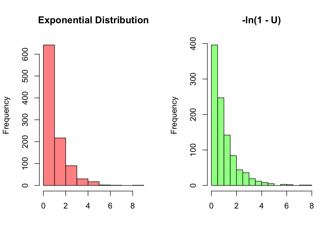

#re-set graphics
par(mfrow = c(1,1))

Hopefully you can now start to see how powerful Universality is. If you are confused about the proof, go up a couple of paragraphs, and if you are still confused about it in practice, go over the example. Think about why this example would be relevant. The CDF we worked with, \(1 - e^{-x}\), is pretty simple, but imagine if we had a random variable with a really complicated CDF and wanted to simulate it on a computer. It’s difficult to envision how to convert that CDF into some kind of distribution we can simulate from, so instead we can use the Universality as we did above and ultimately just simulate the Uniform (which is easy to do). In other words, in the above example we simulated \(U\) a bunch of times (simply generated random numbers between 0 and 1, which any computer could do), and plugged these values into \(-ln(1 - U)\), and this whole new random variable followed the distribution we wanted (Exponential, which we will learn about later).

This result is the first major result of Universality. The second result says something pretty similar, but essentially going in the opposite direction: given a random variable \(X\) that has a CDF \(F\), then \(F(X)\) (plugging \(X\) into it’s own CDF) follows a Standard Uniform Distribution \(Unif(0,1)\). That is, mathematically, \(F(X) \sim Unif(0,1)\). It’s intuitive that \(F(X)\) can only take on values 0 to 1, since the CDF returns a probability, but it is incredible that it is Uniform. You might be confused about what it looks like to plug a random variable into it’s own CDF: consider the example above. Plugging in \(X\) would just make the CDF look like \(1 - e^{-X}\). It’s key here again to remember the difference between \(X\) and \(x\). As usual, \(X\) is random, while \(x\) is simply a constant that the random \(X\) crystallizes to.

Let’s consider an example in R. Recall again the Exponential distribution, which we will learn more about later but are simply using now for these examples. We can generate many values from this distribution (which takes one parameter, \(\lambda\)) with rexp, and then plug this vector of values into the CDF with the pexp command. The resulting graph, incredibly, is Uniform on the interval 0 to 1.

#generate the r.v., an Expo(1)
X = rexp(1000, 1)

#plot F(X)
hist(pexp(X, 1), col = rgb(0, 0, 1, 1/2),
     main = "F(X)", xlab = "")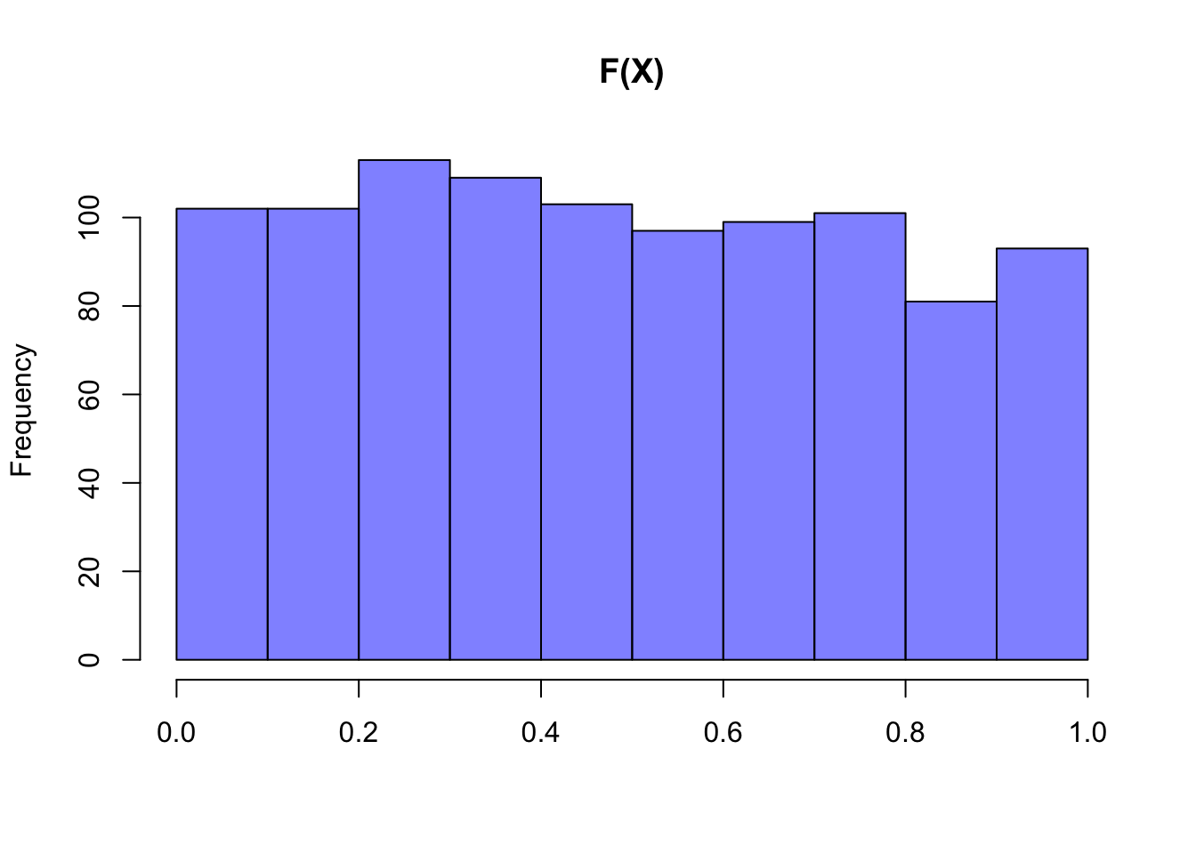

We’re going to discuss the second result Universality a little less, as it is probably the less applicable of the two. In practice, it can be used to check if a random variable is valid; you can plug it into it’s own CDF and see if it follows the Standard Uniform (if it doesn’t, something is wrong).

Normal

This is likely the he most famous and most important distribution in all of Statistics. Also called the “Gaussian Distribution,” the Normal is associated with the distinct bell-shaped curve that you’ve likely seen many times before. We will be using this distribution more than any other, so it’s important to familiarize yourself with it now.

The chief reason why the Normal Distribution is so important is because of a result called the Central Limit Theorem (CLT), probably the most widely used theorem in all of Statistics. For now, we can discuss the general gist: that adding up lots of i.i.d.* random variables eventually leads to a Normal distribution. You may remember seeing that the distribution of sample means from any sort of population becomes Normal as you take more and more samples. So, the overarching idea is that in the end, everything becomes Normal, and this is probably why you’ve seen this bell curve distribution at some point in your travels: because normality is everywhere! We are going to explore the CLT further in Chapter 9.

• We have not yet formalized what i.i.d. means, but it will become a very important term. It stands for Identically and Independently Distributed, which basically means random variables are independent but have the same distribution. Think about flipping two quarters once, separately; they are independent, but have identical distributions (in this case, \(Bern(.5)\) if we’re counting the number of heads).

So, that’s why we care so much about the Normal. You could even think of the CLT as the Story of the Normal Distribution, and you can always think of it as the bell curve that appears when you add up a bunch of random variables. It’s governed by two parameters: a mean, \(\mu\), and a variance, \(\sigma^2\) (by conventional, we let \(\sigma\) be the standard deviation, and we write the variance as the square of this). So, if you want to say something is Normally Distributed with mean \(\mu\) and variance \(\sigma^2\), you could write \(X \sim N(\mu,\sigma^2)\).

Like we define \(Unif(0, 1)\) as the ‘Standard Uniform,’ there is a ‘Standard’ Normal that is often useful and applicable. This is just a Normal centered at 0 (since the Normal is symmetric, that means the mean is 0, because the mean is always at the center) with a variance of 1, or \(N(0,1)\). We often, by conventional notation, call the Standard Normal \(Z\), such that \(Z \sim N(0,1)\).

Let’s start by finding the PDF of \(Z\). You can have the first part for free: the PDF will have a \(e^{-z^2/2}\) term (this gives the nice, smooth, symmetric bell curve), and the rest will be a constant (that is, does not include \(z\)). Knowing that the Normal can take on any value from \(-\infty\) to \(\infty\) (this is the support), can we find the value of the constant? Well, since the PDF must integrate to 1 over the entire support to be a valid PDF, we can just find this integral: \(\int_{-\infty}^{\infty} e^{-z^2/2}dz\). It’s an ugly integral that requires a trick (multiplying by itself and converting to polar coordinates) but eventually we get that this integrates to \(\sqrt{2\pi}\). Since the whole PDF must integrate to 1, then, we can multiply by the constant \(\frac{1}{\sqrt{2\pi}}\) to cancel everything to 1. So, the entire PDF \(f(z)\) is \(\frac{1}{\sqrt{2\pi}}e^{-z^2/2}\) (for the Standard Normal).

We already saw that the Standard Normal has a mean of 0 and a variance of 1, and you can check these with LoTUS. Simply compute the integral \(\frac{1}{\sqrt{2\pi}}\int_{-\infty}^{\infty} ze^{-z^2/2}dz\), which is \(z\) times the PDF, to find the expectation. This should come out to 0 (in fact, you don’t even have to do the integral out. this is an odd function because \(f(-x) = -f(x)\), and odd functions integrate to 0 over these bounds). Then, since we know \(E(Z) = 0\), \(Var(Z) = E(Z^2) - E(Z)^2 = E(Z^2)\). You can find \(E(Z^2)\) by plugging in \(z^2\) to the integral we just did and integrating (we won’t consider it here because it’s just repetitive calculus; the point is to mention another example where LoTUS is useful).

Finally, we get to the CDF, which again gives the cumulative density below a certain point. If we want to find the CDF of \(Z\), we just have to integrate the PDF of a standard normal up to a constant \(t\) (again, we use an arbitrary letter for the constant so as not to mix the bound up with the random variable). Also, it’s worth mentioning that the Standard Normal and its CDF are so common that it actually has a Greek symbol for shorthand notation: \(\Phi\) (capital phi). So, instead, of \(F(z)\), we have \(\Phi(z)\), such that:

\[\Phi(t) = \frac{1}{2\pi} \int_{-\infty}^{t} e^{-z^2/2}dz\]

So, we’re integrating up to the point \(t\), which of course gives the cumulative density below \(t\) for the Standard Normal (again, don’t be thrown by the \(t\), it’s just a dummy variable because we don’t want to have a \(z\) in the integral and also have it as one of the bounds).

The point is, don’t be nervous if you see a \(\Phi\) in practice. In fact, let’s hammer down what it means with some examples. What should \(\Phi(0)\) equal? Well, this is just asking for the cumulative density below the point 0 in a Standard Normal. Since a Standard Normal has a mean 0 (and is thus centered around 0) and is symmetric, exactly half of the density should be above and half should be below 0. So, \(\Phi(0) = .5\) (that is, the mean of the Normal is right in the middle of the distribution). What about \(\Phi(10^{100})\)? Well, since nearly the entire Standard Normal distribution is below this value (yes, there are small non-zero parts that stretch all the way out there since the support goes from \(-\infty\) to \(\infty\), but obviously it’s a very small amount of density), this should approximately be 1. A similar argument goes for \(\Phi(-10^{100})\); since nearly all of the Normal is above this value, this should be pretty much 0. However, since the distribution is symmetric, \(1 - \Phi(-10^{100}) = \Phi(10^{100})\), which is kind of interesting; in general, \(1 - \Phi(-c) = \Phi(c)\).

In fact, we can go a bit further with the Standard Normal CDF via the 68-95-99.7 Rule, which you’ve likely seen if you’ve taken AP Statistics in high school. It says that, for a Normal Distribution , about \(68\%\) of the distribution falls within 1 standard deviation of the mean (i.e., plus-or-minus one standard deviation), about \(95\%\) falls within 2 standard deviations of the mean, and about \(99.7\%\) falls within 3 standard deviations of the mean. This is pretty useful for the Standard Normal because, of course, the standard deviation is 1 (variance is 1 and the square root of 1 is 1). So, what this rule says for the Standard Normal is that \(68\%\) of the distribution lies between -1 and 1, \(95\%\) between -2 and 2, and \(99.7\%\) between -3 and 3.

Let’s practice a little more, then. What does \(\Phi(1) - \Phi(-1)\) equal? This is just giving the cumulative density between -1 and 1, which we know from above is roughly .68. How about \(\Phi(2)\)? Well, we know that \(95\%\) of the data falls between -2 and 2, and since the distribution is symmetrical, about \(47.5\%\) on each side of the mean. Since \(\Phi(2)\) includes the entire bottom half of the distribution and the 47.5 of the top \(50\%\), we get about \(\Phi(2) = .5 + .475 = .975\) (this is approximate, of course, but pretty close). Anyways, you get the gist: using the 68-95-99.7 Rule, you can roughly estimate densities for the Normal Distribution.

It’s easy to perform these types of CDF calculations using R. Consider this chunk of code, which uses pnorm, a function for the CDF of a Normal distribution, to explore the 68-95-99.7 rule and even plot the CDF over the support to show the smooth curve. We don’t specify values for the mu and sigma parameters, meaning that the function defaults to the Standard Normal (mean of 0 and variance of 1). Note that R takes in the standard deviation as an argument, not the variance.

#half of the Normal is below 0
pnorm(0)

## [1] 0.5

#68-95-99.7 Rule
pnorm(1) - pnorm(-1); pnorm(2) - pnorm(-2); pnorm(3) - pnorm(-3)

## [1] 0.6826895

## [1] 0.9544997

## [1] 0.9973002

#plot the CDF
plot(seq(from = -3, to = 3, length.out = 100), pnorm(seq(from = -3, to = 3, length.out = 100)),
     xlab = "x", ylab = "P(X <= x)", main = "CDF of X where X ~ N(0, 1)",
     type = "p", pch = 16)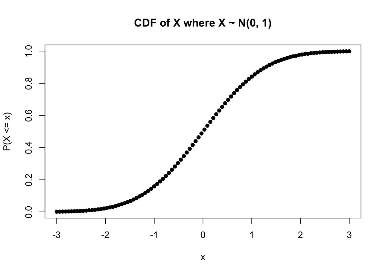

Of course, there are Normal random variables other than the Standard Normal; those that don’t have a mean of 0 and a variance of 1. However, it can often be useful to think of these other Normal Distribution in terms of the Standard Normal, since the CDF of a Standard Normal is so common and easy to work with.

That is, we can create any Normal Distribution from the Standard Normal by shifting and stretching it via location and scale transformations. In math terms, we can make any Normal Distribution \(X\) with mean \(\mu\) and variance \(\sigma^2\) with the following transformation:

\[X = \mu + \sigma Z\]

We think of \(\mu\) as the location, since the Normal is always centered around the mean, and \(\sigma\) the scale, since it ‘stretches’ out the distribution (more or less variance makes it wider or narrower).

How come \(X\) here, though, has expectation \(\mu\) and variance \(\sigma^2\)? First, let’s find the Expectation. By linearity and other properties of expectation (recall that \(E(c) = c\) if \(c\) is a constant, since a constant does not change and thus ‘on average’ it is just itself):

\[E(X) = E(\mu + \sigma Z) = E(\mu) + E(\sigma Z) = \mu + \sigma E(Z) = \mu\]

Since the mean of \(Z\) is 0, or \(E(Z) = 0\). Let’s solve the variance now. To complete this calculation, we need to learn new facts about variance: the variance of a sum of independent variables is the sum of the variances of the individual random variables. That is:

\[Var(X + Y) = Var(X) + Var(Y)\]

If \(X\) and \(Y\) are independent.

From here, we know that the variance of a constant is 0 (the number 7, for example does not vary at all, it’s always 7), and \(Var(cX) = c^2Var(X)\) for any constant \(c\) (think of how we define variance for intuition on this fact), we do:

\[Var(X) = Var(\mu + \sigma Z) = Var(\mu) + Var(\sigma Z) = \sigma^2 Var(Z) = \sigma^2\]

Since the variance of \(Z\) is 1, or \(Var(Z) = 1\).

So, we’ve just proven that \(X\) has mean \(\mu\) and variance \(\sigma^2\). However, although we know that \(X\) is a random variable with this mean and variance, we don’t necessarily know the distribution of \(X\). Is \(X\) Uniform? Is it Geometric? to answer this question, we need an important result.

Concept 4.1: Linear Combination of Normals

If we start with a Normal random variable and add or multiply a constant, the new random variable is Normally distributed. Further, if we add independent Normal random variables together, the sum is also Normally distributed.

With this result, we can say with confidence that \(X\) is Normal (and we have already found the mean and variance). In general, what we actually did is create ‘any’ Normal Distribution we want, just by transforming the Standard Normal (that is, you can stretch and shift the bell curve however you like, but it is still a bell curve). We can go the opposite way, transforming any Normal Distribution we have into a Standard Normal, as well. This is pretty useful because, again, it’s very easy to work with the Standard Normal distribution. Of course, to do this, just solve for \(Z\) in the equation \(X = \mu + \sigma Z\) to get \(Z = \frac{X - \mu}{\sigma}\).

This process, converting a Normal Distribution back to the Standard Normal, is a process called standardization. You might have heard before of “z-scores,” which are essentially values, minus the mean of the distribution and divided by the standard deviation. That’s exactly what standardization is; we’re just converting to a value and seeing where it falls in the Standard Normal distribution, \(Z\), because it’s much easier to work with.

Now that we’ve got that down, what about the PDF of a general Normal Distribution that has mean \(\mu\) and variance \(\sigma^2\)? We can go about finding this via the Standard Normal PDF, which we have already defined. We know that for any Normal distribution with mean \(\mu\) and variance \(\sigma^2\), \(Z = \frac{X - \mu}{\sigma}\). We can then plug in \(\frac{x-\mu}{\sigma}\) for \(z\) in the CDF of a Standard Normal, and then derive that in terms of \(x\) to get the PDF. In Chapter 7, we will learn of another method to find the PDF of \(X\).

When the smoke clears, you get something like this. For a Normal Random Variable with mean \(\mu\) and variance \(\sigma^2\), the PDF \(f(x)\) is given by:

\[f(x) = \Big(\frac{1}{\sigma \sqrt{2\pi}}\Big) e^{\frac{(\frac{x-\mu}{\sigma})^2}{2}}\]

Often you’ll see the \(\sigma^2\) in the numerator of \(e\) float to the denominator next to the 2, but we’ll leave it like this for now so we can see where this comes from (it took the spot of \(z\) in the PDF of a Standard Normal).

Yes, it’s not very elegant, and you can see why we prefer working with the much simpler Standard Normal PDF. In fact, let’s do a quick check to make sure this matches up to what we know is the PDF of a Standard Normal, \(Z\). Well, the mean of \(Z\) is 0 and the variance is 1, so the constant will be \(\frac{1}{\sqrt{2\pi}}\), and the exponent will collapse to just \(\frac{x^2}{2}\).

You can further explore the Normal distribution with our Shiny app; reference this tutorial video for more.

Click here to watch this video in your browser. As always, you can download the code for these applications here.

Hopefully diving into the Normal distribution wasn’t too big a jump. One of the true beauties of Statistics is that the Normal Distribution (much like the Golden Ratio) shows up everywhere in the natural world. It’s important to firmly grasp it here before we ramp up to more complex concepts that rely on knowledge of the Normal.

Exponential

We’ve already worked with the CDF/PDF of this distribution for a few examples, but have not yet formalized it. This will be the third continuous distribution that we learn (after the Normal and the Uniform above). It’s called the Exponential mostly because of the mathematical makeup/functional form of its PDF; you will see in a moment.

The Story of the Exponential is pretty similar to something we have already studied: if \(X \sim Expo(\lambda)\), then \(X\) gives the time waited for the first success in a continuous interval of time, where \(\lambda\) is the rate parameter for the success.

Where have we seen this story before? With the Geometric (and the Negative Binomial which, recall, is a generalized version of the Geometric), which gave the expected time waited for the first success in an interval of discrete trials. That is, while the Geometric might model something discrete, like the number of heads you flip before you flip a tails, the Exponential is the continuous analog: it might measure how much time you have to wait at the bus stop for that first bus to come.

If \(X \sim Expo(\lambda)\), then \(X\) has PDF \(f(x) = \lambda e^{-\lambda x}\). There is not much we can do to intuit this PDF (however, you can see where the name ‘Exponential’ comes from, as we have that \(e\) raised to a power in the PDF) but this is a relatively simple function, and thus we can quickly get the CDF by integrating. Completing this integral yields \(F(x) = 1 - e^{-\lambda x}\). The CDF and PDF are defined for positive values; that is, the support of the distribution is \(x > 0\). This support makes sense when framed in context for the story; you can wait for a bus for a positive amount of time, but you can’t wait for a bus for -5 minutes, for example.

The Expectation of the Exponential is \(\frac{1}{\lambda}\), while the Variance is \(\frac{1}{\lambda ^2}\) (again, you could find these using LoTUS). The expectation is pretty intuitive; if you are waiting for a bus (with arrivals that are exponentially distributed) and the rate of the arrival of the bus is 1 every 10 minutes (that is, \(\lambda = \frac{1}{10}\)), then we would expect a bus to arrive on average every 10 minutes. This is the same as the reciprocal of the rate parameter, which is of course what the expectation is giving us. It’s similar intuition to the expectation of the Geometric, although back then we were working with \(p\) instead of \(\lambda\), and we had discrete time points (i.e., a specific number of flips) instead of a continuous time scale. You can also think about how when \(\lambda\) grows (i.e., we have a higher rate of buses arriving) the average time that we wait for a bus, or \(\frac{1}{\lambda}\), decreases.

Before we delve into some of the nuances of this distribution, you can explore the Exponential with our Shiny app; reference the tutorial video for more.

Click here to watch this video in your browser. As always, you can download the code for these applications here.

Example 4.2: Scaling an Exponential

One interesting, and often useful, characteristic of the Exponential is the outcome you get when scaling the random variable by its rate parameter \(\lambda\). Specifically, if \(X \sim Expo(\lambda)\), then:

\[(\lambda X) \sim Expo(1)\]

We can confirm this by generating values from an Exponential distribution with a specified \(\lambda\) in R using the command rexp.

#define a simple parameter
lambda = 1/5

#generate the r.v.'s
X = rexp(sims, lambda)
Y = rexp(sims, 1)

#compare the histograms; they should match
#set graphic grid
par(mfrow = c(1,2))

#Expo(1)
hist(Y, main = "Expo(1)",
     xlab = "", col = rgb(1, 0, 0, 1/4))

#lamda*Expo(lambda)
hist(lambda*X, main = "Scaled Exponential",
     xlab = "", col = rgb(0, 1, 0, 1/4))

#re-set graphic state
par(mfrow = c(1,1))

So, the rate parameter times the random variable is a random variable that has an Exponential distribution with rate parameter \(\lambda = 1\). Notice, again, that a function of a random variable is still a random variable (if we add 3 to a random variable, we have a new random variable, shifted up 3 from our original random variable). Here, the function is simply the random variable times \(\lambda\).

How is this the case, and how can we show this rigorously? Let’s set \(\lambda X\) equal to \(A\), and then let’s try to find the CDF of \(A\) (as we’ve seen, finding the PDF or CDF of a random variable is a common problem in Statistics, so try to get accustomed to these types of approaches). A good start is to first just write down the definition of what we are trying to find and working from there. We know, by the definition of the CDF, that the CDF is given by \(P(A \leq a)\). We can then plug in \(\lambda X\) for \(A\) to get \(P(\lambda X \leq a)\). Solving for \(X\) (recall that \(\lambda\) is a positive constant) yields \(P(X \leq \frac{a}{\lambda})\). This is just \(\frac{a}{\lambda}\) plugged into the CDF of \(X\), which we already know is \(1 - e^{-\lambda x}\). Plugging in \(\frac{a}{\lambda}\), we get \(1 - e^{-a}\). Remember, this is the CDF of \(A\), which equals \(\lambda X\), and it’s clearly an exponential CDF with rate parameter \(\lambda = 1\) (if \(\lambda\) were 2, for example, we’d have \(-2a\) in the exponent. Instead, we just have \(-a\), implying that the \(\lambda\) we multiplied by is 1). So, we can say with confidence that \(\lambda X \sim Expo(1)\) if \(X \sim Expo(\lambda)\).

We can find the PDF by deriving the CDF to get \(e^{-a}\), and from here it’s actually some pretty easy integration to get the expectation and variance of an \(Expo(1)\) random variable. We know that both the Variance and Expectation are going to come out to 1, based on the formulas we already have (the expectation is \(1/\lambda\) and the variance is \(1/\lambda^2\)), but it’s good practice to convince yourself by using LoTUS. This is also a good way to get the general expectation and variance of an Exponential (you only have to do the integration for \(A\), which is easier than doing the integration for \(X\)). Taking the fact that \(\lambda X = A\) and solving for \(X\) yields \(X = \frac{A}{\lambda}\). Since \(\lambda\) is a constant and we know the variance and expectation of \(A\), we could just find the expectation and variance of \(X\):

\[E(X) = E(\frac{A}{\lambda}) = \frac{E(A)}{\lambda} = \frac{1}{\lambda}\]

If we know that \(E(A) = 1\). For Variance:

\[Var(X) = Var(\frac{A}{\lambda}) = \frac{Var(A)}{\lambda^2} = \frac{1}{\lambda^2}\]

If we know that \(Var(A) = 1\). Of course, this matches the general solution we saw for the mean and variance of an Exponential above.

The main point is to remember that a random variable with an Exponential distribution, times it’s rate parameter \(\lambda\), is simply a random variable with distribution \(Expo(1)\). This is a neat little trick; kind of similar to plugging a random variable into it’s own CDF to get the Standard Uniform (Universality!). Be sure to keep your eyes open for it, since it often greatly simplifies a problem.

Example 4.3: Minimum of Exponentials

Aside from this ‘scaling’ example, the Exponential distribution has another interesting property. Let \(X \sim Expo(\lambda_1)\) and \(Y \sim Expo(\lambda_2)\), where \(X\) and \(Y\) are independent (we will formalize what ‘independent random variables’ mean in Chapter 6; for now, just imagine that knowing what value \(Y\) crystallizes to does not affect what value \(X\) crystallizes to). Now let \(Z = min(X, Y)\). There is a sort of ‘real-world’ intuition behind \(Z\): we know that the story for \(X\) and \(Y\) is that they are ‘waiting times’ (generally, we say that they are waiting times for buses), and now we let \(Z\) be the minimum of these waiting times, so we can think of \(Z\) as the time of the first bus arrival (it doesn’t matter which bus arrives, since \(Z\) just marks the first arrival).

What is the distribution of \(Z\)? Does it have a named distribution that we have worked with? To find the distribution, we can try to find the CDF of \(Z\) and see if this is a CDF that we recognize. By definition, we have:

\[P(Z \leq z) = 1 - P(Z > z)\]

We took the complement of \(P(Z \leq z)\) because it is easier to find \(P(Z > z)\). Let’s consider this probability. If \(Z > z\), and \(Z\) is the minimum of \(X\) and \(Y\), that means that both \(X\) and \(Y\) must be greater than \(z\). That is, we can write:

\[P(Z > z) = P(X > z \cap Y > z)\]

Since \(X\) and \(Y\) are independent (again, we will formalize this later) we can multiply the marginal probabilities:

\[= P(X > z) P(Y > z)\]

We know the CDF of \(X\) and \(Y\), so we can write this in terms of the CDFs:

\[=\big(1 - P(X \leq z)\big) \big(1 - P(Y \leq z)\big)\]

Plugging in to \(P(W \leq w) = 1 - e^{-\lambda \cdot w}\) for \(W \sim Expo(\lambda)\) (i.e., the CDF of \(X\) and \(Y\), since they have Exponential distributions) yields:

\[=e^{-\lambda_1 z}e^{-\lambda_2 z} = e^{-(\lambda_1 + \lambda_2)z}\]

Recall that this gives \(P(Z > z)\), and plugging this in to \(P(Z \leq z) = 1 - P(Z > z)\) yields:

\[P(Z \leq z) = 1 - e^{-(\lambda_1 + \lambda_2)z}\]

Does this look familiar? In fact, it does: it looks like the CDF of a \(Expo(\lambda_1 + \lambda_2)\) random variable. That is, \(Z \sim Expo(\lambda_1 + \lambda_2)\).

This is an interesting result: the minimum of Exponential random variables is itself Exponentially distributed, and the parameter is the sum of the parameters of the original Exponential random variables (we could generalize this fact to the minimum of \(n\) Exponentials, not just 2 Exponentials as we have here). Consider the parameter of the minimum for a moment (the sum of the parameters of the original random variables). Does this parameter make sense? Recall that, for an Exponential random variable, the expectation is the reciprocal of the rate parameter, so a larger rate parameter means a smaller expectation (the higher the rate, the smaller the average wait time). The minimum of Exponentials, then, has a larger rate parameter than the original Exponentials, which means it has a lower expectation; that makes sense, since the time we expect to spend waiting for the first bus to arrive should be lower than the time we expect to wait marginally for each bus (on average, the minimum wait time for any bus to arrive should be smaller than the marginal wait time of any one bus. Intuitively, it is impossible for any one bus to beat the ‘fastest’ arrival time; if a bus ‘beats’ the fastest time, than it just set a new ‘fastest time!’).

Finally, let’s finish up the Exponential distribution by thinking again about its discrete counterpart: the Geometric. What else did we learn about the Geometric that was notable? Well, we know that it is the degenerate case of the Negative Binomial (which counts the number of failures until \(r\) successes), but this isn’t what we’re going to look at for the Exponential, at least not yet. Instead, recall the interesting property of the Geometric distribution: Memorylessness.

As we’ve discussed earlier, the Memoryless property could also be called the “good as new” property: it basically states that, if your distribution is memoryless, you have the same expected value no matter how much time has passed (more broadly, the time you now have to wait follows the same distribution as it did originally). This is especially relevant in terms of the Geometric distribution, remember, because we are waiting until we see a success. Memorylessness says that no matter how long you have been waiting, it’s always ‘good as new’; you should expect to still wait the same amount (and your waiting time has the same distribution going forward).

The property is the exact same for the Exponential distribution, except on a continuous scale. For example, the Geometric distribution’s memorylessness might apply to flipping coins: if you’re waiting for the first time you flip a heads, it doesn’t matter how many tails you have previously flipped, you should still expect the same Geometric distribution as when you started. For the Exponential, which is essentially the continuous version, you could imagine waiting for your food in a restaurant. If the wait time has an Exponential distribution, it is memoryless. So, if on average you will wait 20 minutes, then if you are 3 hours in you should still expect to wait 20 minutes (i.e., you shouldn’t expect it to come sooner based on what has happened in the past). Again, this probably doesn’t hold very much in real life. As we mentioned earlier, the longer you wait for your food at a restaurant, the less time you should usually expect to wait in the future. Sometimes, if you have been waiting for an extremely long time, it usually means something has happened - maybe the chef has quit in frustration after one too many broken whisks - and your success won’t come for an even longer amount of time. Of course, these are tangential, unrelated discussions!

Anyways, this result is usually disheartening for the person waiting, because an Exponential distribution marks time waiting for a success. We’d like to think that if we have been waiting for a while, we’re ‘due’ some sort of success because we’ve made some sort of ‘progress’ by waiting, but unfortunately, if the distribution is truly memoryless, that is not the case. That’s why you might call memorylessness the ‘frustration’ principle (instead of ‘good as new’), based on your perspective!

How did we prove memorylessness earlier on with the Geometric distribution? Well, in words, it basically means that the probability of waiting for some interval of time shouldn’t change given that some time has passed. This would imply that the distribution of waiting time has not changed. In our notation:

\[P(X \geq k) = P(X \geq k + t| X \geq t) \]

You can think of \(k\) as the 20 minutes you would expect to get your food in at the restaurant and the \(t\) as the three hours you have been waiting for it. The left side of the equation, of course, just gives the probability that you wait 20 minutes or more from the beginning. The right side says, given that you have waited for 3 hours, what is the probability that you wait another 20 minutes (in total, \(k + t\) minutes)? If a distribution is memoryless, it doesn’t matter what has happened in the past, and the probability of waiting \(k\) more minutes should always be the same. We can prove this with the Exponential, using the same approach as the Geometric proof:

\[P(X \geq n + k | X \geq n) = \frac{P(X \geq n + k \; \cap \; X \geq n)}{P(X \geq n)}\] \[\frac{P(X \geq n + k)}{P(X \geq n)} = \frac{e^{-\lambda (n + k)}}{e^{-\lambda n}} = e^{-\lambda k}\]

We get \(e^{-\lambda k}\), which is equal to \(P(X \geq k)\), since this is just 1 minus the CDF of an Exponential (recall that \(P(X \geq k) = P(X > k)\) here, because a continuous random variable has probability 0 of taking on any specific value). Again, we can visualize this property in R. We can generate ‘wait times’ from an Exponential distribution using rexp, and then compare the overall histogram to the histogram of ‘wait times’ conditioned on waiting for more than a specific time; the histogram should not change. We can compare this to similar plots for the Normal distribution, which is not memoryless and thus has different histograms for the ‘extra’ wait times!

#replicate
set.seed(110)
sims = 1000

#define simple parameters (n, p for binomial and geometric) and value of k
n = 10
lambda = 1/10
mu = 3
sigma = 1
k = 5

#generate the r.v.s
X = rexp(sims, lambda)
Y = rnorm(sims, mu, sigma)

#graphics
#set graphic grid
par(mfrow = c(2,2))

#overall histogram
hist(X, main = "X ~ Expo(lambda)", xlab = "", freq = FALSE,
     col = rgb(1, 0, 0, 1/4))

#condition
hist(X[X > k] - k, main = "(X - k)|X > k", freq = FALSE,
     xlab = "", col = rgb(1, 0, 0, 1/4))


#overall histogram
hist(Y, main = "Y ~ N(mu, sigma^2)", xlab = "", freq = FALSE,
     col = rgb(0, 1, 0, 1/4))

#condition
hist(Y[Y > k] - k, main = "(Y- k)|Y > k", freq = FALSE,
     xlab = "", col = rgb(0, 1, 0, 1/4))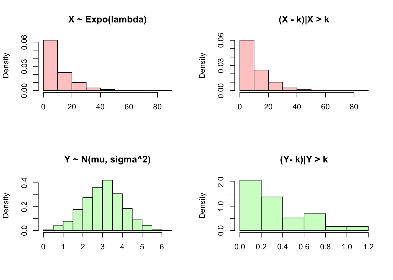

#re-set graphic state
par(mfrow = c(1,1))

Interestingly enough, the Exponential distribution is the only continuous distribution with the memoryless property, similar to how the Geometric distribution is the only discrete distribution with the memoryless property! We can build some final intuition around this result with a visual explanation:

Click here to watch this video in your browser.

Practice

Problems

4.1

Fantasy Sports (especially Fantasy Football) are extremely popular in the United States. Essentially, ‘owners’ (regular citizens) compete by picking the football players that they think will perform the best in a specific set of real-life games. Each football player is assigned a numerical score based on their real-life performance (higher score is better), and the ‘owner’ that scores the most points in aggregate (the sum of all of the football players they picked, or their ‘lineup’) wins.

Imagine that you need to fill two more spots on your ‘lineup’ (pick two more players) and you have two options: you could select Tom Brady (widely considered the greatest player of all time) and Jimmy Graham, or Eli Manning and Rob Gronkowski. By considering historical data, you can reasonably approximate the ‘fantasy points’ that each player will independently score: \(T \sim N(27, 4)\), \(J \sim N(3, 1)\), \(E \sim N(11, 2)\), \(R \sim N(18, 5)\), where \(T\) stands for Tom Brady’s score, etc. (the independence condition is often unrealistic, especially here because Brady and Gronkowski are on the same team, but we will assume independence here). Which option (Brady and Graham, or Manning and Gronkowski) is more likely to score more points? Find the probability of this option scoring more than the other option; you can leave your answer in terms of \(\Phi\).

4.2

1. Is it possible to have two i.i.d. random variables \(X\) and \(Y\) such that \(P(X > Y) \neq 1/2\)?

For the following parts, let \(X, Y\) be i.i.d. \(N(0,1)\).

2. \(E(\Phi(X)) \; \_\_\_ \; \Phi(E(X))\)

3. \(P(X/Y < 0) \; \_\_\_ \; P(\frac{|X - Y|}{\sqrt{2}} < 1)\)

4.3

Imagine that you won in the first round of your diving competition, and now, in the next round, you perform only one dive. The scoring of your dive is as follows: you will be judged by three judges on a scale of 0 to 10 (10 being the best) and the maximum rating given by the three judges will be your score. Unlike the previous problem, ratings are given on a continuous scale; instead of just integers, a judge may give 3.14, for example.

Unfortunately, the judges in this specific competition do not have an eye for the sport at all, and each one independently assigns you a random score between 0 and 10.

1. What is the probability that the first judge gives you the highest score of the group?

2. Let \(H\) be your competition score. Find \(E(H)\).

4.4

1. Let \(X\sim N(0,1)\). What is \(E(X^5)\)?

2. Let \(Y \sim Pois(\lambda)\). Find \(E(\frac{c}{Y + 1})\) where \(c\) is a constant.

3. Let \(Q\) be a Uniform Distribution such that \(Q \sim Unif(0,4)\). Find \(Var(\sqrt{Q})\).

Hint: it may be easier to work in terms of the standard uniform, and the convert.

4.5

Let \(H = 1 - U\), where \(U\) is the Standard Uniform, and \(G\) follow a Gamma Distribution (which we will cover later) with parameters \(\alpha\) and \(\lambda\), PDF \(f(g) = \frac{\lambda^\alpha}{\Gamma(\alpha)}g^{\alpha-1}e^{-g\lambda}\) and CDF \(F(g)\). Find \(E(H - F(G))\).

4.6

Consider a ‘random cube’ generated with side length \(S \sim Unif(0,10)\). Let \(V\) be the volume of the cube. Find \(E(V), \; Var(V)\) as well as the CDF and PDF of \(V\).

4.7

Let \(X \sim N(0, 1)\). For what values of \(b\) does \(E(e^{x^b/2})\) diverge?

4.8

Let \(X\) be a discrete random variable such that the support of \(X\) is \(1,2,...,n\), where \(n > 2\), and \(P(X = x) = \frac{2x}{n(n + 1)}\).

1. Verify that \(P(X = x)\) is a valid PMF.

2. Find \(E(X)\) and \(Var(X)\).

Hint: Feel free to use these facts: \(\sum_{k = 1}^n k = \frac{n(n + 1)}{2}\), \(\sum_{k = 1}^n k^2 = \frac{n(n + 1)(2n + 1)}{6}\), and \(\sum_{k = 1}^n k^3 = \Big(\frac{n(n + 1)}{2}\Big)^2\).

4.9

Imagine a job that pays 1 dollar after the first day, then 2 dollars after the second day, then 4 dollars after the third day, etc., such that the payments continue to double. However, at the end of each day, your boss flips a fair coin, and if it lands tails, you are fired (before you are paid). Let \(X\) be the total, lifetime earnings that you get from this job.

1. Find \(E(X)\), as well as the PMF of \(X\).

2. Based on \(E(X)\), is this a job that you want? Does \(E(X)\) tell the whole story?

4.10

Let \(X \sim Expo(\lambda)\) and \(Y = X + c\) for some constant \(c\). Does \(Y\) have an Exponential distribution? Use intuition about the Exponential distribution to answer this question.

4.11

Let \(X,Y\) be i.i.d. \(N(0, 1)\). Find \(E\big((X + Y)^2\big)\) using the fact that the linear combination of Normal random variables is a Normal random variable.

4.12

1. You plan to try to log on to your email at some random (Uniform) time between 4:00 and 5:00. Independently, the internet will crash sometime between 4:00 and 5:00 and will be unavailable from the time that it crashes to 5:00. What is the probability that you are able to log on to your email (i.e., the computer is not crashed when you log on)?

2. In this part, two ‘break points’ are randomly (Uniformly) and independently selected between 4:00 and 5:00. The internet will not be available between these two points, but will be available for the rest of the hour. What is the probability that the computer is not crashed when you log on?

4.13

Imagine a single elimination tournament with \(2^n\) teams, where \(n \geq 1\). ‘Single elimination’ means that if you lose a game, you are eliminated. You can envision the tournament set-up in simple cases. When \(n = 1\), we have two teams that play each other for the championship. When \(n = 2\), we have four teams; they are split into pairs, and the winner of each pair meets in the championship. The tournament set-up continues to expand in this way as we add teams (see the March Madness tournament for an example where \(n = 6\)).

Imagine for this problem that every team is equally skilled (in real life, this is clearly not a reasonable assumption) such that any random team has equal probabilities of winning or losing against any other random team. Assume games are independent (also not a reasonable assumption in real life). Let \(X\) be the number of games won by the first team.

1. Find \(E(X)\) using LoTUS.

2. Find \(E(X)\) using a symmetry argument.

BH Problems

The problems in this section are taken from Blitzstein and Hwang (2014). The questions are reproduced here, and the analytical solutions are freely available online. Here, we will only consider empirical solutions: answers/approximations to these problems using simulations in R.

BH 4.56

For \(X \sim Pois(\lambda)\), find \(E(X!)\) (the average factorial of \(X\)), if it is finite.

BH 4.59

Let \(X \sim {Geom}(p)\) and let \(t\) be a constant. Find \(E(e^{tX})\), as a function of \(t\) (this is known as the moment generating function; we will see in Chapter 6 how this function is useful).

BH 4.60

The number of fish in a certain lake is a Pois\((\lambda\)) random variable. Worried that there might be no fish at all, a statistician adds one fish to the lake. Let \(Y\) be the resulting number of fish (so \(Y\) is 1 plus a Pois\((\lambda)\) random variable).

1. Find \(E(Y^2)\).

2. Find \(E(1/Y)\).

BH 4.61

Let \(X\) be a Pois(\(\lambda\)) random variable, where \(\lambda\) is fixed but unknown. Let \(\theta = e^{-3\lambda}\), and suppose that we are interested in estimating \(\theta\) based on the data. Since \(X\) is what we observe, our estimator is a function of \(X\), call it \(g(X)\). The bias of the estimator \(g(X)\) is defined to be \(E(g(X)) - \theta\), i.e., how far off the estimate is on average; the estimator is unbiased if its bias is 0.

1. For estimating \(\lambda\), the r.v. \(X\) itself is an unbiased estimator. Compute the bias of the estimator \(T=e^{-3X}\). Is it unbiased for estimating \(\theta\)?

2. Show that \(g(X) = (-2)^X\) is an unbiased estimator for \(\theta\). (In fact, it turns out to be the only unbiased estimator for \(\theta\).)

3. Explain intuitively why \(g(X)\) is a silly choice for estimating \(\theta\), despite (b), and show how to improve it by finding an estimator \(h(X)\) for \(\theta\) that is always at least as good as \(g(X)\) and sometimes strictly better than \(g(X)\). That is, \[|h(X) - \theta| \leq |g(X) - \theta|,\] with the inequality sometimes strict.

BH 5.11

Let \(U\) be a Uniform r.v. on the interval \((-1,1)\) (be careful about minus signs).

1. Compute \(E(U), Var(U),\) and \(E(U^4)\).

2. Find the CDF and PDF of \(U^2\). Is the distribution of \(U^2\) Uniform on \((0,1)\)?

BH 5.12

A stick is broken into two pieces, at a uniformly random breakpoint. Find the CDF and average of the length of the longer piece.

BH 5.16

Let \(U \sim Unif(0,1)\), and \[X = \log\left(\frac{U}{1-U}\right).\] Then \(X\) has the Logistic distribution, as defined in Example 5.1.6.

1. Write down (but do not compute) an integral giving \(E(X^2)\).

2. Find \(E(X)\) without using calculus.

BH 5.19

Let \(F\) be a CDF which is continuous and strictly increasing. Let \(\mu\) be the mean of the distribution. The quantile function, \(F^{-1}\), has many applications in statistics and econometrics. Show that the area under the curve of the quantile function from 0 to 1 is \(\mu\).

BH 5.32

Let \(Z \sim N(0,1)\) and let \(S\) be a random sign independent of \(Z\), i.e., \(S\) is \(1\) with probability \(1/2\) and \(-1\) with probability \(1/2\). Show that \(SZ \sim N(0,1)\).

BH 5.33

Let \(Z \sim N(0,1).\) Find \(E \left(\Phi(Z) \right)\) without using LOTUS, where \(\Phi\) is the CDF of \(Z\).

BH 5.34

Let \(Z \sim N(0,1)\) and \(X=Z^2\). Then the distribution of \(X\) is called Chi-Square with 1 degree of freedom. This distribution appears in many statistical methods.

1. Find a good numerical approximation to \(P(1 \leq X \leq 4)\) using facts about the Normal distribution, without querying a calculator/computer/table about values of the Normal CDF.

2. Let \(\Phi\) and \(\varphi\) be the CDF and PDF of \(Z\), respectively. Show that for any \(t>0\), \(I(Z>t) \leq (Z/t)I(Z>t)\). Using this and LOTUS, show that \(\Phi(t) \geq 1 - \varphi(t)/t.\)

BH 5.36

Let \(Z \sim N(0,1)\). A measuring device is used to observe \(Z\), but the device can only handle positive values, and gives a reading of \(0\) if \(Z \leq 0\); this is an example of censored data. So assume that \(X=Z I_{Z>0}\) is observed rather than \(Z\), where \(I_{Z>0}\) is the indicator of \(Z>0\). Find \(E(X)\) and \(Var(X)\).

BH 5.38

A post office has 2 clerks. Alice enters the post office while 2 other customers, Bob and Claire, are being served by the 2 clerks. She is next in line. Assume that the time a clerk spends serving a customer has the Exponential(\(\lambda\)) distribution.

1. What is the probability that Alice is the last of the 3 customers to be done being served?

Hint: No integrals are needed.

2. What is the expected total time that Alice needs to spend at the post office?

BH 5.41

Fred wants to sell his car, after moving back to Blissville (where he is happy with the bus system). He decides to sell it to the first person to offer at least $15,000 for it. Assume that the offers are independent Exponential random variables with mean $10,000.

1. Find the expected number of offers Fred will have.

2. Find the expected amount of money that Fred will get for the car.

BH 5.44

Joe is waiting in continuous time for a book called The Winds of Winter to be released. Suppose that the waiting time \(T\) until news of the book’s release is posted, measured in years relative to some starting point, has an Exponential distribution with \(\lambda = 1/5\).

Joe is not so obsessive as to check multiple times a day; instead, he checks the website once at the end of each day. Therefore, he observes the day on which the news was posted, rather than the exact time \(T\). Let \(X\) be this measurement, where \(X=0\) means that the news was posted within the first day (after the starting point), \(X=1\) means it was posted on the second day, etc. (assume that there are 365 days in a year). Find the PMF of \(X\). Is this a named distribution that we have studied?

BH 5.50

Find \(E(X^3)\) for \(X \sim Expo(\lambda)\), using LOTUS and the fact that \(E(X) = 1/\lambda\) and \(Var(X) = 1/\lambda^2\), and integration by parts at most once. In the next chapter, we’ll learn how to find \(E(X^n)\) for all \(n\).

BH 5.51

The Gumbel distribution is the distribution of \(-log(X)\) with \(X \sim Expo(1)\).

1. Find the CDF of the Gumbel distribution.

2. Let \(X_1,X_2,\dots\) be i.i.d. Expo(1) and let \(M_n = \max(X_1,\dots,X_n)\). Show that \(M_n - log(n)\) converges in distribution to the Gumbel distribution, i.e., as \(n \to \infty\) the CDF of \(M_n - \log n\) converges to the Gumbel CDF.

BH 5.55

Consider an experiment where we observe the value of a random variable \(X\), and estimate the value of an unknown constant \(\theta\) using some random variable \(T=g(X)\) that is a function of \(X\). The r.v. \(T\) is called an estimator. Think of \(X\) as the data observed in the experiment, and \(\theta\) as an unknown parameter related to the distribution of \(X\).

For example, consider the experiment of flipping a coin \(n\) times, where the coin has an unknown probability \(\theta\) of Heads. After the experiment is performed, we have observed the value of \(X \sim \textrm{Bin}(n,\theta)\). The most natural estimator for \(\theta\) is then \(X/n\).

The bias of an estimator \(T\) for \(\theta\) is defined as \(b(T ) = E(T) - \theta\). The mean squared error is the average squared error when using \(T(X)\) to estimate \(\theta\): \[\textrm{MSE}(T) = E(T - \theta)^2.\] Show that \[\textrm{MSE}(T) = \textrm{Var}(T) + \left(b(T)\right)^2.\] This implies that for fixed MSE, lower bias can only be attained at the cost of higher variance and vice versa; this is a form of the bias-variance tradeoff, a phenomenon which arises throughout statistics.

BH 5.57

1. Let \(X_1,X_2, \dots\) be independent \(N(0,4)\) r.v.s., and let \(J\) be the smallest value of \(j\) such that \(X_j > 4\) (i.e., the index of the first \(X_j\) exceeding 4). In terms of \(\Phi\), find \(E(J)\).

2. Let \(f\) and \(g\) be PDFs with \(f(x) > 0\) and \(g(x) > 0\) for all \(x\). Let \(X\) be a random variable with PDF \(f\). Find the expected value of the ratio \[R=\frac{g(X)}{f(X)}.\] Such ratios come up very often in statistics, when working with a quantity known as a likelihood ratio and when using a computational technique known as importance sampling.

3. Define \[F(x) = e^{-e^{-x}}.\]This is a CDF and is a continuous, strictly increasing function. Let \(X\) have CDF \(F\), and define \(W = F(X)\). What are the mean and variance of \(W\)?

BH 5.59

As in Example 5.7.3, athletes compete one at a time at the high jump. Let \(X_j\) be how high the \(j\)th jumper jumped, with \(X_1,X_2,\dots\) i.i.d. with a continuous distribution. We say that the \(j\)th jumper is “best in recent memory” if he or she jumps higher than the previous 2 jumpers (for \(j \geq 3\); the first 2 jumpers don’t qualify).

1. Find the expected number of best in recent memory jumpers among the 3rd through \(n\)th jumpers.

2. Let \(A_j\) be the event that the \(j\)th jumper is the best in recent memory. Find \(P(A_3 \cap A_4), P(A_3),\) and \(P(A_4)\). Are \(A_3\) and \(A_4\) independent?

References

Blitzstein, J. K., and J. Hwang. 2014. Introduction to Probability. Chapman & Hall/CRC Texts in Statistical Science. CRC Press. https://books.google.com/books?id=z2POBQAAQBAJ.