Chapter 1 Counting

Pat Playjacks: “Hello, Count. And what do you do for a living?”

Count Von Count: “I count.”

We are currently in the process of editing Probability! and welcome your input. If you see any typos, potential edits or changes in this Chapter, please note them here.

Motivation

Despite the trivial name of this chapter, be assured that ‘learning to count’ is not as easy as it sounds. Complex counting problems anchor many probability calculations (i.e., counting the number of favorable outcomes and the number of the total outcomes), making this topic a reasonable place to start.

As this chapter will make clear, counting problems tend to scale in complexity very quickly. However, counting is one of the most satisfying concepts to master; with steady effort and an organized approach, you will soon enjoy the simple beauty of not-so-simple counting.

Sets

We will won’t dive too deeply into set theory here (although it is interesting to note that the word ‘set’ ranks among the words with the most definitions in the English dictionary). However, the notation established in this chapter will be very common throughout the rest of the book, so it is important to familiarize yourself with it early on.

Sets and Subsets - A ‘set’ is defined as a group of objects (i.e., sets can be made up of letters, numbers, names, etc.). A ‘subset’ is defined as a ‘set within a set’; set $A$ is a subset of set $B$ if and only if every element (each object in a set is also called an element) of $A$ is also in $B$.

Empty Set - The set that contains nothing, denoted $\emptyset$.

Union - ‘$A \cup B$’ means, in english, ‘$A$ union $B$.’ This is a shorthand way of saying $A$ or $B$. This set (yes, the union of two sets is itself a set) includes objects in the set $A$, objects in the set $B$ and objects in both sets $A$ and $B$. Picture the union as being the entire Venn Diagram of $A$ and $B$.

Intersection - ‘$A \cap B$’ means, in english, ‘$A$ intersect $B$.’ This is a shorthand way of saying $A$ and $B$. Picture the middle, overlapping part of the Venn Diagram of $A$ and $B$.

Complement - You will probably see this in two ways: $A^c$ and $\bar{A}$ both mean, in english, “$A$ complement.” This is a shorthand way of saying when $A$ does not occur. This set is made up of everything not in $A$.

Disjoint Sets - Sets that do not have any overlap. You could say that the intersection of disjoint sets is the empty set (there are no elements in the intersection of two disjoint sets, which is by definition the empty set).

Partition - Imagine a set $A$, and then imagine subsets $A_1,A_2,A_3,A_4...A_n$. If these subsets are disjoint (so they do not overlap) and cover all possible outcomes in $A$, they partition the set $A$. Consider the trivial example of partitioning in politics: for the sake of simplicity, imagine for a moment that the two major American political parties, Democrats and Republicans, are the only parties in politics. Given this simplification, we can say that $D$, the set of all Democrat politicians, and $R$, the set of all Republican politicians, partition the set of $P$, or all American politicians. That’s because one politician can’t be both Democrat and Republican (there’s no overlap, so the sets are disjoint) and Democrats and Republicans (in this simplified example; in real life we know that there are many other parties, although they are less popular) cover the entire set of American politicians.

So far, these topics should be relatively easy to grasp. Let’s solidify these concepts with an example. Remember, the Union, Intersection and Complements of sets are all sets themselves.

Example 1.1 (Statistics at Harvard)

Let $A$ be the set of all Statistics majors at Harvard, and let $B$ be the set of all students that live in Winthrop (a specific House, or dorm, at Harvard; students are distributed among 12 residential Houses, much like they are distributed among the 4 Houses at Hogwarts).

What is the Union of the sets $A$ and $B$? Well, in english, this means $A$ or $B$, so the Union is the set comprised of all Statistics majors who are non-Winthrop students, all Winthrop students who are non-Statistics majors, and all Winthrop students who are Statistics majors. Again, it may be helpful to think of a simple Venn Diagram here, with the two circles labeled ‘Statistics major at Harvard’ and ‘Winthrop Student at Harvard.’

What is the Intersection of $A$ and $B$? Well, in english, this means $A$ and $B$, so the Intersection is the set of all Winthrop students that are also Statistics majors. Visually, picture the overlap in the Venn Diagram. Note that the Union of $A$ and $B$ includes the Intersection of $A$ and $B$; formally, the Intersection is a subset of the Union.

What is the Complement of $A$? Well, in english, this means when $A$ does not occur, so this is the set of all people that are not Harvard Statistics majors.

Finally, let’s think of an example of a disjoint set. Let $P$ be the set of all USA Presidents in history, and $M$ be the set of all people named ‘Matt.’ These two sets are disjoint because they don’t overlap: no Matt has ever been President/no President has ever been named Matt. Officially, they are disjoint because their intersection is the empty set: there is no one in the set ‘USA President and named Matt.’ Visually, this Venn Diagram would consist of two circles that do not overlap.

Naive Probability

To this point, you might be wondering about the title of this chapter. Why does counting, something that sounds so trivial, have a place in this book? Like most concepts we will discuss, it all starts with probability.

Concept 1.1 (Naive Definition of Probability):

The probability of an event occurring, if the likelihood of each outcome is equal, is:

\[P(Event) = \frac{number \; of \; favorable \; outcomes}{number \; of \; outcomes}\]

When we are working with probabilities, our notation will be $P(A)$. In english, this means ‘the Probability that event $A$ occurred.’ So, if $A$ is the event of flipping heads in one flip of a fair coin, then $P(A) = .5$. The above, then, is just notating ‘the probability of an event occurring.’ We will frequently use the set notation discussed in the previous section when working with probabilities, which is why that section was placed first!

This ‘Naive Definition’ is a reasonable place to start, because it’s likely how you have calculated probabilities up to this point. Of course, this is not always the correct approach for real world probabilities (hence the name ‘naive’). For example, imagine a random person running for President of the United States. Using the naive definition of probability, their probability of winning the election is .5; one favorable outcome (winning) divided by the total number of outcomes (winning or losing). Clearly this is a simplified approach; different outcomes often have different probabilities associated with them, so it’s important to realize when the naive definition does and does not apply. In the President case, the ‘losing’ outcome is much more likely, so the naive ‘weighting’ scheme does not apply.

Anyways, we often apply the naive definition (correctly, hopefully) automatically: if someone asks you the probability that a fair die rolls a 6, you would say $\frac{1}{6}$ because you quickly reason that there are six outcomes (rolls 1 to 6) and one that is favorable (rolling a 6), so the overall probability is just $\frac{1}{6}$. In this example, it’s very easy to count the number of favorable outcomes and number of total outcomes; however, counting the number of outcomes can quickly become much more complex (as we soon will see). That is why this chapter is necessary: to count the number of total and favorable outcomes, as outlined in the formula above, for very complicated problems. We’ll now dive into some tools that are useful for counting outcomes in certain, specific scenarios.

Concept 1.2 (Multiplication Rule):

To understand the Multiplication Rule, visualize a process that has multiple steps, where each step has multiple choices. For example, say that you are ordering a pizza. The first ‘step’ is to select a size, and this ‘step’ has multiple ‘choices’ or ‘outcomes’: small, medium, large, etc. The next ‘step’ is to pick toppings, and again you have multiple ‘choices/outcomes’: pepperoni, sausage, peppers, etc. Another step might be delivery or no delivery. You can see how this problem grows, and counting the total number of outcomes can become tedious.

The idea here is that we would like to count the number of possible pizzas you could order (i.e., one possibility is ‘small mushroom delivery,’ another is ‘large pepperoni not delivery,’ etc.) in a structured way, since we will need to be able to count these types of outcomes for naive probability problems (for example, what’s the probability that a randomly ordered pizza is a large and has sausage? We first need to count how many possible pizzas there are, or the denominator in the formula for naive definition of probability). So, the multiplication rule states that, in a process where the first step has $n_1$ choices, the second step has $n_2$ choices, all the way up to the $r^{th}$ step that has $n_r$ choices, the total number of possible outcomes is just the multiplication of the choices: $n_1n_2...n_r$.

Let’s solidify this concept with the pizza example. Say that you have 3 choices of size: small, medium and large. You then have 4 choices of toppings: pepperoni, meatball, sausage, and extra cheese. Your final choice is delivery or pickup. All in all, you have these three sets of choices:

Size (small, medium, or large)
Topping (pepperoni, meatball, sausage, or extra cheese)
Order Type (delivery or pickup)

Using the multiplication rule, we can easily count the number of distinct pizzas that you could possibly order. Since there are 3 choices for size, 4 choices for toppings, and 2 choices for pickup, we simply have $3\cdot4\cdot2 = 24$ different pizza options (applying the formula from above, we have $r = 3$, $n_1 = 3$, $n_2 = 4$ and $n_3 = 2$).

Now that we have counted the total of number of possible pizzas, it is easy to solve various probability problems. For example, consider finding the probability of ordering a large sausage if you randomly order a pizza: there are 2 favorable outcomes where you get a large sausage (large sausage not delivered and large sausage delivered) and 24 total outcomes/pizzas, so the probability is $\frac{2}{24} = \frac{1}{12}$. Note that we are randomly ordering a pizza, so that each of the possible 24 pizzas has an equal chance of being selected; this allows us to continue to work in a naive framework.

This is far faster than writing out all of the possible combinations by hand, and 24 combinations isn’t even that extensive; imagine if we had 10 options for each choice! The multiplication rule can greatly simplify a problem.

Let’s use R to generate all of these combinations and see if the empirical result matches our analytical work.

#define the vectors for size, topping and order
size = c("S", "M", "L")
topping = c("pepperoni", "sausage", "meatball", "extra cheese")
order = c("deliver", "pick-up")

#keep track of the pizzas
pizzas = character(0)

#iterate over each value for each variable
for(i in 1:length(size)){
  for(j in 1:length(topping)){
    for(k in 1:length(order)){
      
      #create a pizza
      pizzas = rbind(pizzas, c(size[i], topping[j], order[k]))
    }
  }
}

#print out the pizzas; should have 24
pizzas

##       [,1] [,2]           [,3]     
##  [1,] "S"  "pepperoni"    "deliver"
##  [2,] "S"  "pepperoni"    "pick-up"
##  [3,] "S"  "sausage"      "deliver"
##  [4,] "S"  "sausage"      "pick-up"
##  [5,] "S"  "meatball"     "deliver"
##  [6,] "S"  "meatball"     "pick-up"
##  [7,] "S"  "extra cheese" "deliver"
##  [8,] "S"  "extra cheese" "pick-up"
##  [9,] "M"  "pepperoni"    "deliver"
## [10,] "M"  "pepperoni"    "pick-up"
## [11,] "M"  "sausage"      "deliver"
## [12,] "M"  "sausage"      "pick-up"
## [13,] "M"  "meatball"     "deliver"
## [14,] "M"  "meatball"     "pick-up"
## [15,] "M"  "extra cheese" "deliver"
## [16,] "M"  "extra cheese" "pick-up"
## [17,] "L"  "pepperoni"    "deliver"
## [18,] "L"  "pepperoni"    "pick-up"
## [19,] "L"  "sausage"      "deliver"
## [20,] "L"  "sausage"      "pick-up"
## [21,] "L"  "meatball"     "deliver"
## [22,] "L"  "meatball"     "pick-up"
## [23,] "L"  "extra cheese" "deliver"
## [24,] "L"  "extra cheese" "pick-up"

#count total number of large sausages; should get 2
#   we divide by 3 because rows are length 3, and we want
#   to convert back to number of rows (i.e., number of pizzas)
length(pizzas[pizzas[ ,1] == "L" & pizzas[ ,2] == "sausage"])/3

## [1] 2

Now let’s try to build some intuition as to why the multiplication rule works. Imagine flipping a fair coin and simultaneously rolling a fair, 6-sided die and marking down the result as one outcomes (i.e., $H6$ means we flipped heads and rolled a 6). Using the multiplication rule, it is easy to count the number of possible outcomes: there are two outcomes to the coin flip and 6 possible outcomes to the die roll, so there are $6 \cdot 2 = 12$ possible outcomes. Now, consider why this makes sense. Imagine ‘locking in’ the coin as a ‘Heads’: there are then 6 possible outcomes, Heads and every roll of the die. Now imagine ‘locking in’ the coin as a ‘Tails’: as before, there are 6 outcomes, Tails and each roll of the die. Of course, these two sets together represent all 12 of the possible outcomes, and we can envision this process as a sort of multiplication: when we ‘locked in’ the results of the coin, we essentially had 2 sets (the number of sides on the coin) of size 6 (the number of sides on the die), so we multiplied these numbers for the total number of outcomes. If we had a coin with more sides (ignoring the fact that it wouldn’t be a ‘coin’ anymore) we would still be performing a multiplication (just imagine ‘locking in’ the potential outcomes for the coin, one at a time). This concept extends to processes with more steps (you can think of just ‘locking in’ multiple coins, for example) and thus we have the multiplication rule.

Anyways, we could easily make our pizza problem from earlier much larger, as we hinted at above (selecting from 20 different toppings, etc.). However, we could also make the problem much more complicated: what if you could order multiple toppings? What if you wanted to order multiple pizzas, with the constraint that no two pizzas are identical? It is unclear how the multiplication rule would neatly apply to these paradigms. In fact, to answer these questions, we need to learn more about counting.

Concept 1.3 (Factorial):

You’ve likely seen this before: a number followed by an exclamation point. As you probably know, 5! doesn’t mean that 5 is excited. Instead, it means $5! = 5\cdot4\cdot3\cdot2\cdot1$, or the the product of all positive integers less than or equal to 5.

You may have used the factorial for simple arithmetic calculations, but we are introducing it here in the context of counting. How could this formula be an effective tool for solving counting problems? Earlier, we considered the problem of counting the number of outcomes for a process with multiple steps, where each step has multiple choices (the multiplication rule). Consider now the problem of counting the number of ways to order elements; specifically, the number of ways to order the letters A, B, and C. We will define a specific ‘arrangement’ or ‘order’ as a permutation (i.e., $ABC$ is one permutation), so here we are trying to count the total number of permutations.

You could likely figure this out by just writing out all of the permutations:

\[\{ABC, ACB, BAC, BCA, CAB, CBA\}\]

It’s clear that there are 6 permutations (they are all listed above, and there is no other way to order the three letters). However, you might not always be able to write the permutations out so conveniently: what if you had to do the same for all 26 letters in the alphabet? In that case, if you didn’t feel like writing out the 26 letters over and over and over, you could use the factorial for a more elegant solution. Since there are three distinct letters in our original example, the number of permutations when ordering A,B and C is 3! (which cleanly comes out to $3\cdot2\cdot1 = 6$, an answer that we showed to be correct above by writing out all of the permutations).

So, the factorial can be used to count permutations. Let’s build some intuition as to why this holds: think about actually ordering the letters A,B,C. There are three ‘slots’ that the letters could take: they could either be the first letter in the sequence, the second letter or the third letter (i.e., for the permutation $BAC$, $B$ is the first letter, $A$ is the second letter and $C$ is the third letter). How many different letters can we pick for the first ‘slot’ (i.e., how many letters can we pick to be the first letter in the sequence)? Well, since no letters have been picked yet, there are 3 choices (we can pick A, B or C). How about the second slot? Since we know that 1 letter has been picked for the first slot (A, B or C, it doesn’t matter which) there are now 2 letters left that can go in the second slot. What about the last slot? We know 2 letters have already been picked for the first two slots, so there is only 1 remaining letter.

Since we want the total number of permutations, we employ the multiplication rule (notice how the concepts are already building on themselves; we use the multiplication rule to understand the factorial) and multiply each of the descending ‘numbers of letters left,’ which is the same as taking the factorial of 3. So, if we asked the same question but this time wanted to know how many ways there are to order the entire alphabet, the answer would be $26! = 4.03 \cdot 10^{26}$. Clearly, employing the same brute force method from above (writing out all of these permutations) would be near impossible. If you could write one permutation every second, it would still take over $3 \cdot 10^{18}$ years to write all of the permutations, much longer than the current age of the known universe.

We can confirm this concept by counting all of the possible orderings of the letters A through G with some code in R. There are $7! = 5040$ permutations, so finding the combinations with a brute force method (i.e., writing them all out) is not desirable. A computer, however, can generate the combinations quickly. Here, we will use the permn function from the combinat package (we will see other ways to generate these types of combinations later in this chapter; note that we use combinat::permn, which is our way of telling R to use the permn function from the combinat package; there are other packages that have different functions named permn, so we have to specify which one we want!).

#generate all of the possible permutations
perms = combinat::permn(c("A", "B", "C", "D", "E", "F", "G"))

#look at the first few permutations
head(perms)

## [[1]]
## [1] "A" "B" "C" "D" "E" "F" "G"
## 
## [[2]]
## [1] "A" "B" "C" "D" "E" "G" "F"
## 
## [[3]]
## [1] "A" "B" "C" "D" "G" "E" "F"
## 
## [[4]]
## [1] "A" "B" "C" "G" "D" "E" "F"
## 
## [[5]]
## [1] "A" "B" "G" "C" "D" "E" "F"
## 
## [[6]]
## [1] "A" "G" "B" "C" "D" "E" "F"

#should get factorial(7) = 5040
length(perms)

## [1] 5040

Anyways, despite this long-winded explanation, hopefully it is clear that the factorial can be used (by employing the multiplication rule) for counting ways to order, or permute, objects. This allows us to solve more complex counting problems, but we now move to a concept that will expand our horizons even further.

Concept 1.4 (Binomial Coefficient):

This is perhaps the most useful counting tool we will see in this chapter. It is represented by $n \choose{x}$, which in english is pronounced ‘$n$ choose $x$.’ The full formula, defined in terms of factorials (which we just learned about; again, notice how we need previous concepts to define new concepts), is:

\[{n \choose x} = \frac{n!}{(n-x)! \; (x!)}\]

When we learned about the multiplication rule and the factorial, we learned that these formulas gave us a way to solve some sort of counting problem. The same holds true for this concept. Quite simply, the binomial coefficient gives the number of ways that x objects can be chosen from a population of n objects.

Perhaps the best way to visualize this type of problem is counting the number of ways to form committees out of a larger group. Say you have a population of 300 parents at the local elementary school, and you want to choose 10 parents to be a part of the PTA (Parent Teacher Association). Since we have a population $n=300$ and we want to choose $x=10$ parents from the population, ${300 \choose 10} = 1.4 \cdot 10^{18}$ gives the number of ways that we can pick 10 parents from the pool of 300, or the number of combinations possible for the PTA committee. Clearly, this number is quite large, which means that listing out the possible combinations would not be feasible (note that we define one possible iteration - i.e., one possible committee - as a combination, like we defined a permutation above as one possible ordering of objects).

Again, similar to the factorial and the multiplication rule, it’s not immediately clear how the binomial coefficient correctly counts the number of outcomes in this specific situation (choosing a committee out of a group of people). Let’s break it down with a manageable example.

Say we have the 5 letters $A,B,C,D,E$, and we want to find out how many ways there are to select 3 letters from this set of 5 letters (some of the possible combinations are $\{ABC, BCD, AEC\}$, etc.). You can frame this in terms of the PTA example above: in this case, we just have $n = 2$ parents and we want to select a committee of $x = 3$ parents.

We already know from the definition of the binomial coefficient that the number of combinations is ${5 \choose 3}$, but we haven’t yet discussed the intuition behind this result. Let’s review the full formula for the binomial coefficient $\frac{n!}{(n-x)! \; (x!)}$, or in this case, plugging in $n = 5$ and $x = 3$, $\frac{5!}{(5-3)! \; (3!)}$, to gain some intuition.

Let’s start from the top (literally and figuratively). The numerator $5!$ gives us the number of ways we can organize the letters A,B,C,D and E (it turns out there are 120 ways, since $5\cdot4\cdot3\cdot2\cdot1 = 120$). However, we aren’t asking for the number of ways that we can order the entire set (the permutations), but the number of ways we can choose a certain amount of letters out of the entire set (the combinations). Therefore, this $5!$ is counting permutations like ACDBE and EDCBA, where we only want the combinations with 3 letters, not all 5 (from the problem statement, we’re only choosing 3 letters for our ‘committee’). Instead, we can think about this sequence of 5 letters (one permutation) as a sequence of 3 letters followed by a sequence of 2 letters. Of course, we only want the sequence of 3 letters and could care less about the 2 letters left over, so we have to divide out those extra two letters that we don’t want.

So, if someone is putting together the 5 letters in a random order, we essentially want to stop them at 3 letters (this will define a committee of 3). How can we count in this way? Well, once they have picked three letters to order out of all five letters (like BEC or DAB) they still have $2!$ possible ways that they can order the remaining letters. If they start with ABC, for example, there are $2!$, or $2\cdot1 = 2$, ways to order the remaining letters: DE and ED. The $5!$, then, is overcounting what we want (groups of three) by a factor of 2!, so we must divide the $5!$ by $2!$, which is of course just $(n-x)!$ or $(5-3)!$.

Therefore, we are starting from the number of ways that we can pick the 5 letters in a row, and then adjusting for the fact that we are picking the entire sequence of 5 letters instead of the 3 letters that we asked for by dividing by $(5-3)!$ or $2!$, the letters we don’t care about. It’s sort of like dividing by the number of ways to not choose 3 letters.

That accounts for $n!$ in the numerator and the $(n - x)!$ in the denominator of the binomial coefficient. What about the $x!$ term? Well, where have we left off in our counting structure? After dividing, we’ve just found the number of ways to choose sets of 3 letters out of the 5 letters. However, we are still overcounting in some fashion.

The key here is that order doesn’t matter (a concept we will explore further in this chapter). The division we just did, $\frac{5!}{(5-3)!}$, spits out the number of ways to choose 3 letters from A,B,C,D,E. This happens to come out to 60 (you can type factorial(5)/factorial(5 - 3) in R to prove it). We’ll start to write out the combinations. See if you notice any patterns:

\[ABC,ACB,BCA,BAC,CAB,CBA,ABD,ADB,BDA,BAD,DBA,DAB...\]

Did you catch it? Here, we have written out 12 of the 60 combinations.

Consider the first six: $\{ABC,ACB,BCA,BAC,CAB,CBA\}$. They all have the same letters in them: A, B and C, the only factor that makes them unique is the order that they are presented in (i.e., ABC and ACB have the same letters but in a different order). This is the same for the second set of six combinations above, but with the letters A, B and D. They are permuted differently but have the same combination.

Think back to one of the original examples for the binomial coefficient: picking people for committees. Does it matter which order you pick the people for the committees in? No, it does not; as long as the same people are in a committee, it does not matter what order we picked them in.

Therefore, if A, B and C are people, then the committees $\{ABC\}$ and $\{ACB\}$ are the exact same committee. That is, picking Alec, then Bob, then Carl forms the same committee as picking Carl, then Alec, then Bob. Since we don’t really care which order they are selected in, this method again overcounts committees: the set of 6 permutations with the letters A, B and C should only count for 1 committee combination.

How do we fix this? Again, by dividing out to adjust for overcounting. Since there are $3!$ ways to permute the people in the committee, but again, we don’t want to count these ways, we have to divide by $3!$. You can see the intuition in this case: since $3! = 6$, and we just saw that 6 committees should have ‘boiled down’ to 1. You can further convince yourself of this by the fact that there are 10 total permutations of these ‘false 6’ (two of which we wrote out) because there are 10 ways to group the letters ABCDE (ABC, ABD, ABE, ACD, ACE, ADE, BCD, BCE, BDE, CDE) and within each group $3! = 6$ ways to permute the letters (which we don’t want to count in this case).

So, we divide by the 3!, which completes the formula $\frac{5!}{(5-3)! \; (3!)}$. It comes out to 10 (in fact, we wrote out the complete answer at the end of the last paragraph) which means that there are 10 ways to select 3 letters from ABCDE, or 10 ways to form a committee of size 3 from 5 different people. We learned that this formula adjusts for over-counting in selecting unnecessary orderings (dividing by $(5-3)!$ to get us down to just permutations of 3) and over-counting in giving extra ordering combinations (ABC and ACB are the same in this problem structure).

We can confirm this result in R by generating all possible committees of size 3 from 5 total people using the combinations function, which is in the gtools package (again, we use gtools::combinations to tell R that we want the function combinations specifically from the gtools package).

#generate the committees (people labeled 1 to 5)
committees = gtools::combinations(n = 5, r = 3)

#should get choose(5, 3) = factorial(5)/(factorial(3)*factorial(2)) = 10 committees
committees

##       [,1] [,2] [,3]
##  [1,]    1    2    3
##  [2,]    1    2    4
##  [3,]    1    2    5
##  [4,]    1    3    4
##  [5,]    1    3    5
##  [6,]    1    4    5
##  [7,]    2    3    4
##  [8,]    2    3    5
##  [9,]    2    4    5
## [10,]    3    4    5

A final exercise to solidify our understanding of the binomial coefficient is to consider ${n \choose x}$ when $x > n$. Thus far, we have implicitly assumed $n \geq x$; after all, we are choosing $x$ objects from a population of $n$ objects, so we should have that the population of objects is larger than the group we hope to choose. Consider, then, the case when $x > n$; this problem is explored further in the practice problems at the end of this chapter (as always, you can quickly check your intuition in R with the choose function).

Anyways, we have now learned how to count processes with multiple steps, as well as how to permute and combine objects. From these simple tools, a world of complexity opens up.

Sampling Table

Here is a convenient way to arrange the results that we have discussed thus far (and extend our knowledge to cover more ground), from Blitzstein and Hwang (2014).

	Order Matters	Order Doesn’t Matter
With Replacement	\[n^k\]	\[{n+k - 1 \choose k}\]
Without Replacement	\[\frac{n!}{(n-k)!}\]	\[{n \choose k}\]

This table will allow us to think more deeply about the concepts we have learned in this chapter. Before we dive into each section, let’s think about what Order and Replacement mean.

If ‘Order Matters,’ then two outcomes that have the same elements in a different order are counted as different outcomes; if ‘Order Doesn’t Matter,’ they are counted as one outcome. For example, if ‘Order Matters,’ then ABC, CAB, BAC are counted as three separate outcomes, and if ‘Order Doesn’t Matter’ they are counted as one outcome (since they all have the letters A, B and C in them, and it doesn’t matter how they are arranged). Order matters when we care about permutations (recall that permutations count the number of ways to arrange objects). Generally, order doesn’t matter when we consider combinations: in the committee example, at least, you get the same committee no matter what order you picked people in.

If we are picking ‘With Replacement,’ that just means that after we select an object, we put it back into the population and it can be picked again. For example, if we are drawing cards out of a deck and we are sampling with replacement, we put the card back after we draw it and we could then pick it again. Without replacement, we would take the card out of the deck after we picked it, meaning we could not pick the card again (it also makes the deck a little smaller, obviously. We can only draw without replacement from a 52-card deck, well, 52 times. After that, there are no more cards left!).

The entries in the Sampling Table, then, count the number of ways to choose objects from a group of objects (here, we choose $k$ objects from $n$ objects). Adjusting the constraints of ‘Order’ and ‘Replacement’ allows us to define how we choose the objects and essentially moves us around the table. Now, let’s explore these different ways to count.

First, let’s consider the top left box in the Sampling Table. This box wants us to count the number of ways to select $k$ objects from $n$ objects with replacement where order matters. When we put objects back in after picking them (with replacement) we will always be picking from $n$ objects (since we start with $n$ objects, and we replace each object we take). Since every single time we will have $n$ options and we are picking $k$ times, we simply have to multiply $n$ by itself $k$ times (by the multiplication rule), or $n^k$. Since order actually matters, we aren’t overcounting anything and don’t have to divide by some factor to correct this: we don’t want to throw out the permutations with different orders, because order matters.

The next best box to think about is the bottom right: the binomial coefficient. Here, order does not matter and we are taking objects out of the population after we sample them (without replacement) so it makes sense to just use the binomial coefficient ${n \choose k}$, since this counts the number of ways to select $k$ objects from a population of $n$ objects where we are not replacing the objects and the order that we select the objects in is not important (for more on why the binomial coefficient has these properties, see the explanation in the previous section).

From here, we move to the bottom left box. This looks almost identical to the binomial coefficient except that it doesn’t have the extra $k!$ term in the denominator. That’s because, if you recall, we include that $k!$ to divide out the overcounting that results from differences in order (i.e., if order doesn’t matter, we want ABC, ACB, CBA, CAB, BCA, BAC to count as 1 outcome, so we divide by 3!). However, since we are in the column ‘Order Matters,’ we actually want to count these different permutations, so we do everything the same way but do not divide by $k!$ so as to keep in these specific permutations.

Finally, we will refer to the top right box as the ‘Bose-Einstein’ result, and it is probably the trickiest box to master. Here, we are sampling with replacement, and order doesn’t matter. Let’s consider an explanation adapted from Blitzstein and Hwang (2014). Imagine that we are trying to count the number of ways to put $k$ balls in $n$ boxes, where the balls are all the same (indistinguishable) but the boxes are different (distinguishable). First, consider why this satisfies the constraints ‘sampling with replacement’ and ‘order doesn’t matter.’ Imagine that we put the balls into the boxes one by one. We can think of ‘putting a ball in a box’ as ‘sampling’ a box; whenever we ‘sample’ a box, we just add a ball to it! Since we can put as many balls in any box as we want (i.e., once we put a ball in a box, or ‘sample’ that box, we can still ‘sample’ it again) we are essentially sampling boxes with replacement. Since the balls are identical, order doesn’t matter. These two outcomes are the same: ball 1 goes in box 1 and ball 2 goes in box 2 vs. ball 2 in box 1 and ball 1 in box 2. It only matters how many balls end up in each box, not the order that they were placed there, since the balls are indistinguishable!

At this point, we should just be convinced that this ‘ball-box’ scheme (putting identical balls in non-identical boxes) is the same as sampling with replacement such that order doesn’t matter. Now, we turn to discussing why ${n+k - 1 \choose k}$ actually counts the number of ways to perform this type of sampling. Again, we’re going to borrow an explanation from Professor Blitzstein (you can read a more thorough discussion from Professor Blitzstein here). Imagine when $n = 3$ and $k = 5$ (we have 3 boxes and 5 balls). One possible permutation of the sampling is below:

\[| \bullet \bullet \bullet | \bullet | \bullet |\]

As you might be able to guess, this diagram shows a sample where we have 3 balls in the first box, 1 ball in the second, and 1 ball in the third (the $\bullet$ marks are balls, and the $|$ marks are the walls of the boxes. The walls ‘overlap,’ so the second $|$ in the sequence above, reading from left to right, is the right-hand wall for the first box and the left-hand wall for the second box).

Now that we can visualize the sampling process in this way, we can actually just count the ways to legally permute the above diagram (this is equivalent to counting the number of ways to perform the sampling, since we already argued that this ‘box and balls’ scheme is the same in structure to the type of sampling we are interested in). The only thing that stays fixed are the two bars on the end (the diagram wouldn’t make sense if there was a $\bullet$ on the end, because we would have one box that wasn’t closed). In this case, after we fix two bars on the ends, we now have 2 bars left over and 5 balls to rearrange within themselves. There are 7 spots for these 7 objects (bars and balls), so if they were all different there would be 7! ways to permute them (by the concept of the factorial). However, the balls are all identical to each other, and the bars are identical to each other (the boxes aren’t identical in the problem, but in this diagram, swapping bars does not change the boxes). Therefore, we have 7! ways to arrange the objects, and then we have to divide out by 5!, the number of ways to arrange the balls within themselves, and 2!, the number of ways to arrange the bars within themselves. This comes out to $\frac{7!}{5!2!}$, which is the same as ${7 \choose 5}$. Notice how $n + k - 1 = 7$ and $k = 5$; extending to the general case, then, there are ${n+k - 1 \choose k}$ ways to perform this sampling (the $-1$ comes from the fact that we have one less ‘movable bar’ - that is, bars that are not on the ends of the diagram and thus cannot be moved - than boxes in our diagram).

The Sampling Table may be the most important concept in this chapter because it links together the tools we’ve learned; therefore, it’s extremely important to understand the concepts and various sampling constraints. You can interact with the ‘Permutations’ Shiny app to solidify your understanding; reference this tutorial video for more.

Click here to watch this video in your browser. As always, you can download the code for these applications here.

Ultimately, the best way to develop understanding for the entries in the Sampling Table is to practice. Consider the following problem, which can be solved with methods discussed in this chapter. Both analytical solutions (i.e., with pencil and paper) and empirical solutions (i.e., simulations in R) are presented.

Example 1.2 (Call Me Maybe):

Most responsible iPhone users choose a ‘passcode’ for their device: a chosen security code to prevent others from using their phone. Passcodes are 4 digits long and are can consist of the integers 0,1,…,9.

How many possible passcodes are there?
Define a ‘unique’ passcode as a passcode with 4 distinct digits (i.e., 2947 is unique but 3391 is not). How many unique passcodes are there?
Define an ‘ascending’ passcode as a passcode where each digit is equal to or larger than the previous digit (i.e., 1489 and 1122 are ascending passcodes, but 1948 is not). How many passcodes are both unique and ascending?
How many ascending (not necessarily unique) passcodes are there?
Describe how your answers to this problem relate to the Sampling Table.

Analytical Solution:

There are 10 possible selections for each of the 4 digits (0,1…, or 9). By the multiplication rule, there are $10^4$ possible passcodes.
There are 10 possible choices for the first digit; for the second digit, we can pick any digit except for the digit we picked first, meaning we have 9 choices. Continuing in this way, we have $10 \cdot 9 \cdot 8 \cdot 7 = \frac{10!}{6!}$ possible passcodes.
Every possible set of digits that we sample without constraint for a passcode can be ordered to make an ‘ascending passcode,’ but there is only one of these orders that is ‘legal’ (i.e., ascending order. If you sample the digits 4, 6, 9 and 2, the only ordering that makes an ascending passcode is 2469). So, we can adjust our answer to (b) by dividing out all of the $4!$ possible orders for the unique passcode (only one is ascending). This yields $\frac{10!}{6! 4!} = {10 \choose 4}$.
This is the Bose-Einstein paradigm; we are sampling digits from 0 to 9 with replacement (the passcode need not be unique), and order doesn’t matter (i.e., for any 4 digits we sample, there is one correct ascending order to put them in, so sequences with the same digits in different orders ‘represent’ only one outcome). Therefore, there are ${10 + 4 - 1 \choose 4}$ of these passcodes.
We start in the top left of the Sampling Table in part (a) and then move counterclockwise. In part (a), we sample digits with replacement (i.e., you can have the passcode 9999) and order matters (i.e., the passcode 2299 is different from the passcode 9922). In part (b), when we introduce uniqueness, order still matters, but now we are sampling without replacement (i.e., once you select a 9, you can not select a 9 again). In part (c), in addition to uniqueness, which determines sampling without replacement, we essentially mandate that order doesn’t matter: if we sample 9218 and 8192, both ‘represent’ the passcode 1289 (the ‘ascending’ rule forces a single order; ‘order not matters’ here means that we will arrange the numbers into a single order). Sampling without replacement with order not mattering gives the binomial coefficient. Finally, in part (d), we remove the unique condition (so sample with replacement) but keep the ascension condition (so order does not matter), which gives us Bose-Einstein.

Empirical Solution:

Since 4-digit phone numbers from 10 possible digits are computationally difficult to work with, we consider only a 4-digit passcode from 6 digits. The permutations function in the gtools package generates permutations of a given size from a given vector, and we can dictate if we want to include repeats (i.e., unique sequences) with the repeats.allowed argument.

### part a. ###
#should get 6^4 = 1296
dim(gtools::permutations(n = 6, r = 4, repeats.allowed = TRUE))[1]

## [1] 1296

### part b. ###
#should get factorial(6)/factorial(2) = 360
dim(gtools::permutations(n = 6, r = 4, repeats.allowed = FALSE))[1]

## [1] 360

## part c. ##
#find the unique passcodes
uniques = gtools::permutations(n = 6, r = 4, repeats.allowed = FALSE)

#create unique and ascending passcodes
uniques.ascending = apply(uniques, 1, function(x) sort(x))

#orient the matrix (the function t() just transposes a matrix; flips it on it's side)
uniques.ascending = t(uniques.ascending)

#create a data frame
uniques.ascending = data.frame(uniques.ascending)

#remove duplicates; should get choose(6, 4) = 15
dim(unique(uniques.ascending))[1]

## [1] 15

## part d. ##
#find all passcodess
passcodes = gtools::permutations(n = 6, r = 4, repeats.allowed = TRUE)

#create ascending passcodes
ascending = apply(passcodes, 1, function(x) sort(x))

#orient the matrix (the function t() just transposes a matrix; flips it on it's side)
ascending = t(ascending)

#create a data frame
ascending = data.frame(ascending)

#remove duplicates; should get choose(6 + 4 - 1, 4) = 126
dim(unique(ascending))[1]

## [1] 126

You can further solidify your understanding of these concepts with this problem that counts the number of possible pairings in $2n$ people. We also consider this problem in the practice section of this chapter.

Click here to watch this video in your browser.

Story Proofs

This is the last bit of counting that we’ll cover in this chapter, and it’s sort of just like it sounds: proving something by means of a story. Basically, you explain something with words instead of with algebra.

Story proofs are really at the heart of this book; we hope to, above all, present an engaging narrative. While mathematical, rigorous proofs are important, being able to tell a story about a specific concept can be much more elegant and even promote a deeper understanding of the material. You can use story proofs for just about anything, and here we will demonstrate their use in a counting example.

Example 1.3 (Symmetry of the Binomial Coefficient):

Prove, with a story, that:

\[{n \choose k} = {n \choose n - k}\]

This is a relatively straightforward example, and also pretty useful in a pinch: it’s often referenced as the symmetry of the binomial coefficient. You may be able to immediately see that plugging in the algebraic definition of a binomial coefficient makes this proof trivial:

\[\frac{n}{k! \cdot (n - k)!} = \frac{n}{(n - k)! \cdot k!}\]

The above is clearly true; the only difference between the two sides is that the denominators are ordered differently, and we know that $a \cdot b = b \cdot a$. However, we want to prove this relation by using a story instead of mathematical rigor.

Here, a good way to think about this equation is to consider the number of ways to pick a team of $k$ people out of $n$ total people. The left side of the equation, ${n \choose k}$, gives the number of ways to pick the team of size $k$ (we should be comfortable with this concept at this point). The right side, ${n \choose n - k}$, gives the number of ways to pick the people not on the team (if $k$ people are on the team, then $n - k$ people are not on the team), which is the same thing as picking who is on the team. That is, since there are only two options, (1) on the team or (2) not on the team, picking who is on the team also picks who is off the team (the people who weren’t picked) and vice versa. So, the two sides are equal, as we saw with the algebraic proof above.

Let’s ground this result with an example. Imagine that there are 7 kids on the playground, but only 5 are going to be picked for the basketball team at recess. Picking the 5 that are on the team is the same as picking the 2 that are not on the team; if you pick 2 that will not be on the team, we know that the other 5 must be on the team! Think of it as splitting the population into two different groups; if we observe who is in one group, we know with a certainty who is in the other group.

We can further visualize this in R by considering a specific example where we generate committees of size 2 and size 1 from a population of 3 people.

#generate the committees (people labeled 1 to 5)
committees2 = gtools::combinations(n = 3, r = 2)
committees1 = gtools::combinations(n = 3, r = 1)

#print the sets of the two committees
committees2; committees1

##      [,1] [,2]
## [1,]    1    2
## [2,]    1    3
## [3,]    2    3

##      [,1]
## [1,]    1
## [2,]    2
## [3,]    3

Consider the output; the first 3x2 matrix represents all committees of size 2 (i.e., the first row means that we have a committee made up of person 1 and 2). The second 3x1 matrix is similar, but instead the rows are of length 1, since the committees are of size 1.

Now imagine comparing the two outputs. The first row of the committees2 matrix maps to the third row of the committees1 matrix; that is, picking the first and second person to be on the committee of size 2 is the same as picking the third person to NOT be on the committee. The matrices have the same number of rows, of course, because picking who is on the committee is equivalent to picking who is off the committee, by the story above!

Example 1.4:

Prove, with a story, that:

\[k{n \choose k} = n{n - 1 \choose k - 1}\]

Again, this is not difficult to show with algebra. Plugging in the definition of the binomial coefficient:

\[= \frac{kn!}{k! \cdot (n - k)!} = \frac{n(n - 1)!}{(k - 1)!\cdot (n - k)!}\]

\[= \frac{n!}{(k - 1)! \cdot (n - k)!} = \frac{n!}{(k - 1)!\cdot (n - k)!}\]

However, again, we want to consider a story. The best way to envision this relationship is again with picking committees; this time, though, imagine that you are picking a committee of size $k$ people out of a population of $n$ people and you are selecting one president for the committee. So, there are two selections: picking the $k$ people to be in the committee, and then picking the one person from the $k$ people in the committee to be the president.

First, let’s consider the left side of the equation. Here, we have the basic ${n \choose k}$, which of course gives the number of ways to select the committee of $k$ people. However, once we’ve done this, we have another selection: picking the president of the committee. Since there are $k$ people in the committee, we have $k$ options to choose from, and thus by the multiplication rule we just multiply the first choice, picking the committee, or ${n \choose k}$, by the second choice, or picking the president from the committee of $k$ people. By this logic, the left hand side of the equation counts what we are interested in: the number of ways to pick a committee with a president.

We now have to prove that the right hand side of the equation gives the same thing. Let’s imagine that this time, instead of picking the committee first, we select the president and then the committee. So, if we are picking the president first from the population, we of course have $n$ choices (we can pick anyone in the whole population). Then, after picking the president, we have to select the committee, and since there are $n -1$ people left (we have already taken one out to be president) and we need $k-1$ more people in the committee (we already have the president) we just multiply by ${n -1 \choose k -1}$. So, by the multiplication rule, we multiply the first choice of picking the president from $n$ people by the second choice of picking the rest of the $k-1$ sized committee from the $n-1$ people.

So, then, the only difference between the two sides is that the left side picks the committee first and then the president from the committee, while the right side picks the president from the population and then selects the rest of the committee. Clearly, switching the order of these selections does not change the number of ways to choose a committee with a president, and our story holds: both sides of the equation are counting the same thing.

We can confirm our intuition in R by considering a committee of size 3 drawn from a population of size 4, with one president.

#label people 1 to 4
people = 1:4

#first, we do the president-first approach
#initialize the committees
committees1 = character(0)

#iterate through potential presidents
for(i in 1:length(people)){
  
  #generate the new committes, with i as the president
  new.committees = cbind(i, gtools::combinations(n = length(people) - 1, r = 2, v = people[-i]))
  
  #add on to existing committees
  committees1 = rbind(committees1, new.committees)
}

  
#remove column names
colnames(committees1) = c("", "", "")



#second, we do the committee-first approach; initialize here
committees2 = character(0)

#generate all of the committees, without presidents
new.committees = gtools::combinations(n = 4, r = 3)

#iterate through the committees and add presidents
for(i in 1:dim(new.committees)[1]){
  
  #pick each person as president
  for(j in 1:3){
    
    #add the committee
    committees2 = rbind(committees2, c(new.committees[i, j], new.committees[i, -j]))
  
  }
}

#remove column names
colnames(committees2) = c("", "", "")

#print the two groups of committees; should be the same size
#   the first person is president in each case
#we should have k*choose(n, k) = 3*choose(4, 3) = 12 total
committees1

##                  
##  [1,] "1" "2" "3"
##  [2,] "1" "2" "4"
##  [3,] "1" "3" "4"
##  [4,] "2" "1" "3"
##  [5,] "2" "1" "4"
##  [6,] "2" "3" "4"
##  [7,] "3" "1" "2"
##  [8,] "3" "1" "4"
##  [9,] "3" "2" "4"
## [10,] "4" "1" "2"
## [11,] "4" "1" "3"
## [12,] "4" "2" "3"

committees2

##                  
##  [1,] "1" "2" "3"
##  [2,] "2" "1" "3"
##  [3,] "3" "1" "2"
##  [4,] "1" "2" "4"
##  [5,] "2" "1" "4"
##  [6,] "4" "1" "2"
##  [7,] "1" "3" "4"
##  [8,] "3" "1" "4"
##  [9,] "4" "1" "3"
## [10,] "2" "3" "4"
## [11,] "3" "2" "4"
## [12,] "4" "2" "3"

Symmetry

This is not a topic exclusive to probability, Statistics in general, or even this chapter within this book; it is simply a tool that can help solve complicated problems. Symmetry, when used correctly, can be both very powerful and extremely elegant.

Nearly everyone is familiar with the colloquial concept of ‘symmetry,’ but it’s not always easy to apply symmetry to actual problems. In general, symmetry can greatly simplify a complex problem, reducing the structure to something much more manageable; in the context of this book, think of it as a problem solving tool (it is such a powerful problem solving tool that we gave it a section all to itself!). It’s probably best to discuss an example where symmetry can apply.

Example 1.5 (Spades)

Imagine a standard, well-shuffled, 52 card deck of cards. You are dealt four cards from the deck at random. On average, how many spades will you get in this four card deal?

Analytical Solution: At first glance, this seems like a difficult problem. We can be dealt anywhere from 0 to 4 spades, and there are many possible combinations for each (i.e., there are many ways to be dealt 0 spades). We might consider taking a ‘weighted average’ (we will formalize this concept in later chapters); that is, find the probability that we are dealt 0 spades, then 1 spade, etc., and then multiplying the probability by the number of spades found (i.e., the probability of finding 1 spade times 1, plus the probability of finding 2 spades times 2, etc.). This is certainly possible, but it seems like a lot of work.

Instead, let’s use symmetry. We are being dealt 4 of the 52 cards in the deck; we can think of there being 13 groups of 4 cards each in this deck (i.e., cards 1 through 4 are one group, then cards 5 through 8, etc.), since $4 \cdot 13 = 52$, and we simply own the first ‘group’ of 4 cards. We know that the total number of spades totaled across all of these groups is always 13; there are 13 spades in the deck, and these 13 groups account for the entire deck. By symmetry, we know that, on average, every group will get the same amount of spades. So, since there are 13 groups that represent 13 spades between them, and every group has the same average number of spades, each group must get 1 spade on average (it wouldn’t make sense if certain groups of 4 tended to get spades more often). So, in your four-card deal, you expect one spade.

Empirical Solution:

#replicate
set.seed(110)
sims = 1000

#create a deck; define spades as 1, everything else as 0
deck = c(rep(1, 13), rep(0, 52 - 13))

#keep track of the number of spades we sample
spades = rep(NA, sims)

#run the loop
for(i in 1:sims){
  
  
  #deal the four card hand
  hand = sample(deck, 4, replace = FALSE)
  
  #see how many spades we got
  spades[i] = sum(hand)
}

#should get 1
mean(spades)

## [1] 1.012

The key argument in the analytical solution above, of course, is the ‘symmetry’ argument. Consider what we argued: by symmetry, every ‘group’ of 4 cards should expect the same number of spades on average. Does this make sense? Well, since the deck is randomly shuffled, and the groups are arbitrary (i.e., we don’t deal in any sort of biased way to any of the groups), this must be true. That is, there’s no information in the problem that tells us that the groups should be at all different in terms of the number of spades that they are dealt on average.

It’s a strange argument, but tough to dispute and, as we saw, powerful. We were pondering performing a probability calculation instead of using this symmetry argument; this might have been feasible in this case, but what if we had a much larger deck and were dealt a much larger hand? Here, the elegant symmetry argument is much easier to implement. In general, it’s more generalizable and intuitive to understand.

Throughout this book, you will notice that symmetry arguments often provide extremely effective approaches to solving problems. Symmetry is a theme that will surface for nearly every topic we cover, which is why we include it in the first chapter. For a final example, consider another problem where symmetry can be used effectively:

Click here to watch this video in your browser.

Practice

Problems

1.1

Consider a standard, well-shuffled deck of cards. What is the probability that the 4 Aces are all adjacent? Here, define ‘adjacent’ as taking four consecutive positions; i.e., the 1st, 2nd, 3rd and 4th cards in the deck. The definition is not circular: the first and last cards in the deck are not considered adjacent.

1.2

There are eight schools in the Ivy League (Harvard’s athletic conference): Harvard, Yale, Princeton, Brown, Columbia, Dartmouth, Cornell and Penn. The academic rankings of these schools is often a topic of interest and controversy. How many different ways are there to rank these schools?
Sometimes, Harvard, Yale and Princeton are referred to as the ‘Big 3,’ and are often grouped together as schools because of their extensive similarities. If indeed these three schools were identical - that is, the ordering ‘Harvard Yale Princeton’ is taken as identical to the ordering ‘Yale Princeton Harvard’ - how many ways would there now be to rank the Ivies?

1.3

You are tasked with dividing 20 kids into two kickball teams at recess. Games have been very even in the past, so you decide to make things more interesting by giving 1 team 9 players and the other team 11 players. How many ways could you make these teams?
Can you write your answer to part (a) in a different format?
After the first game, the team with 9 people complained because of the inherent disadvantage. For the second game, you decide to again put 10 people on each team. How many ways can you do this?

1.4

For this problem, assume a normal, well-shuffled 52 card deck. You are dealt 5 cards (called a ‘hand’) randomly from the deck.

The best hand in Poker is a royal flush: the 10, Jack, Queen, King and Ace of the same suit. What is the probability that you are dealt a royal flush?
What is the probability that you are dealt a 3 of a kind (getting exactly 3 of the same value, like three jacks)?

1.5

Tony has 5 meetings to schedule this business week (Monday through Friday). Define a ‘permutation’ here as a schedule of meetings by day (i.e., two meetings on Monday, one meeting on Thursday and two meetings on Friday is one permutation). If meetings are indistinguishable, how many permutations are there if Tony does not want to have all five meetings on a single day?

1.6

Consider a state that has 5 different counties (a ‘county’ is a collection of towns: for example, the town Burlington, Connecticut is in Hartford County), and each county has 6 different towns. Imagine that you want to visit every town in the state; however, you don’t want to visit each county more than once (you can fly from any town to any other town in the state). Define a permutation as one specific ordering of the 30 visits you make (one to each town). How many permutations are there?

1.7

Imagine a game of tic-tac-toe where the players randomly select a blank space each turn to make their move. If $X$ goes first, what is the probability that $X$ wins on their third move?

1.8

Imagine a modified game of tic-tac-toe called ‘tic-tac-max.’ The only difference in tic-tac-max is that players put down $X$’s and $O$’s until the board is completely filled, not just until someone gets 3 in a row. $X$ still goes first.

Define a permutation as one game sequence; i.e., player 1 puts an $X$ in the top left spot, then player 2 puts an $O$ in the top right spot, etc. Permutations are considered distinct if they are completed in different orders. How many possible permutations are there to play this game?
Define a ‘final board’ as the configuration of the board after each player has put all of their ‘pieces.’ How many possible ‘final boards’ are there?

1.9

(With help from Nicholas Larus-Stone and CJ Christian)

There are $2n$ people. How many ways are there to pair the people up?

For example, if we had four people named $A$, $B$, $C$ and $D$, one permutation would be the pairs $\{A, B\}$ and $\{C, D\}$. A second permutation would be the pairs $\{A, C\}$ and $\{B, D\}$ (one permutation is defined by pairing everyone).

1.10

Imagine the digits $0,1,2,...,9$. How many ways are there to make a three-digit number and seven-digit number from these digits? For example, $\{538\}$ and $\{1246790\}$ as the three- and seven-digit numbers is one permutation; a second permutation is $\{835\}$ and $\{1246790\}$.

1.11

(With help from Juan Perdomo)

Consider these 5 points:

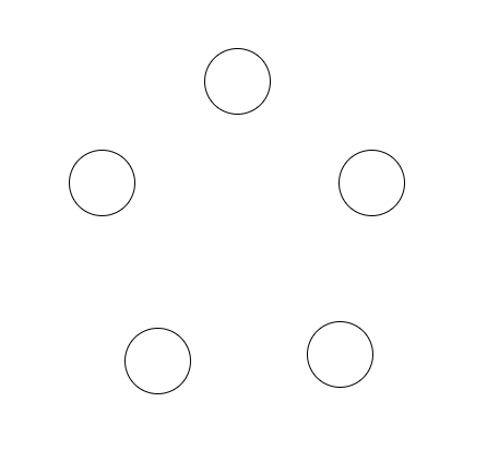
You can make plots like this in Latex here.

Imagine selecting two points at random and drawing a straight line in between the two points. Do this 5 times, with the constraint that you cannot select the same pair twice. What is the probability that the lines and points form a pentagon (i.e., a five-sided, five-angled, closed shape)?

1.12

There are $n$ people, each with a left and a right foot. Each has 2 shoes (one for each foot), so there are $2n$ shoes. Define a ‘permutation’ as an allocation of the $2n$ shoes to the $n$ people, such that the left shoes are on the left feet and the right shoes are on the right feet. If shoes are distinguishable, how many permutations are there?

1.13

Nick claims that, when $n > k$, we have ${n \choose k} {k \choose n} = 1$ because, by the definition of the binomial coefficient, the multiplication in these terms cancel out. Explain why Nick is wrong, using both math and intuition.

1.14

Consider 10 tosses of a fair coin. Let $A$ be the event that you get exactly 5 heads, and $B$ be the event that you get 10 heads.

Compare $P(A)$ and $P(B)$.
Now consider the sequences $HTHTHTHTHT$ and $HHHHHHHHHH$. Compare the probabilities that these sequences occur.
Discuss your results in parts a. and b.

1.15

How many possible 5-letter words are there such that two letters within the word don’t repeat? That is, ‘alamo’ is ok, but ‘aalmo’ is not ok, since the letter ‘a’ repeats.

1.16

(Dedicated to Diana Stone, with help from Matt Goldberg)

There is a restaurant in France called ‘7367.’ After every meal, the waiter rolls four fair, 10-sided dice (numbered 1 through 10). If the dice show a 3, a 6 and two 7’s (in any order) the meal is free.

If you eat at this restaurant once, what is the probability of winning a free meal?
This dice game has made the restaurant very popular, but the manager of the restaurant wants to be able to adjust the game. He would like to present variations of the game for meals that are more expensive (lower probability of winning) and for meals that are less expensive (higher probability of winning).

Keeping the same structure of the dice game, how can you change the ‘winning number’ (i.e., 7367) to suit the manager’s needs, both for higher and lower probabilities of winning? Support your answer both with calculations and intuition.

1.17

Matt, Dan, Alec, Edward and Patrick are settling in for board game night. They pick their spots randomly at a round table with 5 evenly spaced seats. What is the probability that Dan is sitting next to Alec (i.e., he is sitting either directly to the left or right of Alec)?

1.18

Jon Snow and Robb Stark are both in need of knights. There are currently 100 available knights at Winterfell (Jon and Robb’s home); Jon is going to take 10 knights and go North, and Robb is going to take 30 knights and go South.

To avoid potentially displaying favoritism and upsetting the knights of the realm, Jon and Robb will both randomly select their knights. They will flip a coin to determine who goes first; the winner of the coin flip will randomly select his required number of knights (10 or 30) and the loser of the coin flip will then randomly select his required number of knights (10 or 30) from the remaining number of knights (90 or 70).

Jon claims that there are ${100 \choose 10} \cdot {90 \choose 30}$ possible combinations (one single combination marks the knights that Jon took, the knights that Robb took and the knights that stayed back). Robb, though, claims that Jon is off by a factor of 2, because he forgot to account for who picks their knights first (Jon or Robb). Who is correct?
Robb and Jon flip the coin, and Robb wins (the coin lands on the “direwolf” sigil, not the “crow” sigil). However, Robb is not pleased: “Great,” he says, “now I go first, which means I have a higher chance of taking Theon” (Theon is one of the 100 knights and is well known for his ineptitude). Robb and Jon will still both randomly select their knights, as the rules stipulate; does Robb have a higher chance of selecting Theon if he goes first?

1.19

Imagine a game called ‘Cards Roulette.’ The four Aces are removed from the deck and are well shuffled. You take turns with a friend drawing Aces without replacement from the four cards. The first player to draw a red Ace (Hearts or Diamonds) loses.

If you would like to maximize your probability of winning this game, should you go first or second?
Compare this to the Russian Roulette problem from this chapter (click here for a video recap of this problem). Think about how these two problems compare in structure and make an intuitive argument comparing the two solutions.

1.20

Using a story proof, show:

\[{n \choose x} 2^x = \frac{\big(2n\big)\big(2n - 2\big)...\big(2n - 2(x - 1)\big)}{x!}\]

Where $n > x$.

Hint: During police interrogations, it is common to adapt a ‘good cop/bad cop’ strategy. That is, two cops enter the interrogation room, and one cop is the ‘good cop’ (they are nice to the perpetrator to try to get them to open up) while the other cop is the ‘bad cop’ (they are rude and possibly even threatening to scare the perpetrator).

Imagine that you are the police commissioner and you are presented with pairs of cops; the cops come in teams of two. It is your job to select teams, and then assign which cops will be the ‘good cops’ and which cops will be the ‘bad cops’ (each team must have one good cop and one bad cop).

1.21

Define ‘skip-counting’ as an alternative way to count integers. Imagine counting from 1 to 10: a legal ‘skip-count’ is an ascending set of integers that starts with 1 and ends with 10 (i.e., 1-2-5-6-10 and 1-3-10 are both legal ‘skip-counts’).

How many skip-counts are there if we skip-count from 1 to some integer $n > 1$?

1.22

Masterminded by Alexander Lee.

The NFL (National Football League) consists of 32 games that play 17 games amongst each other in a season (each team is given one ‘bye’ week that they have off, but for simplicitly in this problem we will assume all teams play all 17 weeks). By extension, there are 16 games each week (each of the 32 teams plays one other team).

Imagine entering an NFL betting pool with the following rules: you can purchase a single entry for $1, which allows you to pick a game a week until you are wrong. That is, every week, you select a team out of the 32 that you think will win, and if you are correct (the team wins or ties) you advance to the second week. You win if you ‘survive’ for 17 weeks (pick 17 games, one in each week, correctly).

You are allowed to purchase multiple entries; simply imagine that different entries are different chances to play the game. Each entry is independent (you can pick different games, the same games, etc. with different entries) and when an entry fails (you pick a wrong game for that entry) the entry is eliminated, but other entries may continue. If any one of your entries makes it 17 weeks, you win.

What is the least amount of money you have to pay to buy enough entries that allow you to implement a strategy that guarantees victory (at least one entry survives)?

BH Problems

The problems in this section are taken from Blitzstein and Hwang (2014). The questions are reproduced here, and the analytical solutions are freely available online. Here, we will only consider empirical solutions: answers/approximations to these problems using simulations in R.

BH 1.8

How many ways are there to split a dozen people into 3 teams, where one team has 2 people, and the other two teams have 5 people each?
How many ways are there to split a dozen people into 3 teams, where each team has 4 people?

BH 1.9

How many paths are there from the point $(0,0)$ to the point $(110,111)$ in the plane such that each step either consists of going one unit up or one unit to the right?
How many paths are there from $(0,0)$ to $(210,211)$, where each step consists of going one unit up or one unit to the right, and the path has to go through $(110,111)$?

BH 1.16

Show that for all positive integers $n$ and $k$ with $n \geq k$, \[{n \choose k} + {n \choose {k-1}} = {{n+1} \choose k},\] doing this in two ways: (a) algebraically and (b) with a story, giving an interpretation for why both sides count the same thing.

BH 1.18

Show using a story proof that \[{k \choose k} + {k+1 \choose k} + {k+2 \choose k} + ... + {n \choose k} = {n+1 \choose k+1},\] where $n$ and $k$ are positive integers with $n \geq k$. This is called the hockey stick identity.
Suppose that a large pack of Haribo gummi bears can have anywhere between 30 and 50 gummi bears. There are 5 delicious flavors: pineapple (clear), raspberry (red), orange (orange), strawberry (green, mysteriously), and lemon (yellow). There are 0 non-delicious flavors. How many possibilities are there for the composition of such a pack of gummi bears? You can leave your answer in terms of a couple binomial coefficients, but not a sum of lots of binomial coefficients.

BH 1.22

A certain family has 6 children, consisting of 3 boys and 3 girls. Assuming that all birth orders are equally likely, what is the probability that the 3 eldest children are the three girls?

BH 1.23

A city with 6 districts has 6 robberies in a particular week. Assume the robberies are located randomly, with all possibilities for which robbery occurred where equally likely. What is the probability that some district had more than 1 robbery?

BH 1.26

A college has 10 (non-overlapping) time slots for its courses, and blithely assigns courses to time slots randomly and independently. A student randomly chooses 3 of the courses to enroll in. What is the probability that there is a conflict in the student’s schedule?

BH 1.27

For each part, decide whether the blank should be filled in with =, < or > and give a clear explanation.

(probability that the total after rolling 4 fair dice is 21) vs. (probability that the total after rolling 4 fair dice is 22)
(probability that a random 2-letter word is a palindrome) vs. (probability that a random 3-letter word is a palindrome)

BH 1.29

Elk dwell in a certain forest. There are $N$ elk, of which a simple random sample of size $n$ are captured and tagged (“simple random sample” means that all ${N \choose n}$ sets of $n$ elk are equally likely). The captured elk are returned to the population, and then a new sample is drawn, this time with size $m$. This is an important method that is widely used in ecology, known as capture-recapture. What is the probability that exactly $k$ of the $m$ elk in the new sample were previously tagged? (Assume that an elk that was captured before doesn’t become more or less likely to be captured again.)

BH 1.31

A jar contains $r$ red balls and $g$ green balls, where $r$ and $g$ are fixed positive integers. A ball is drawn from the jar randomly (with all possibilities equally likely), and then a second ball is drawn randomly.

Explain intuitively why the probability of the second ball being green is the same as the probability of the first ball being green.
Define notation for the sample space of the problem, and use this to compute the probabilities from (a) and show that they are the same.
Suppose that there are 16 balls in total, and that the probability that the two balls are the same color is the same as the probability that they are different colors. What are $r$ and $g$ (list all possibilities)?

BH 1.32

A random 5-card poker hand is dealt from a standard deck of cards. Find the probability of each of the following possibilities (in terms of binomial coefficients).

A flush (all 5 cards being of the same suit; do not count a royal flush, which is a flush with an ace, king, queen, jack, and 10).
Two pair (e.g., two 3’s, two 7’s, and an ace).

BH 1.40

A norepeatword is a sequence of at least one (and possibly all) of the usual 26 letters a,b,c,…,z, with repetitions not allowed. For example, “course” is a norepeatword, but “statistics” is not. Order matters, e.g., “course” is not the same as “source.”

A norepeatword is chosen randomly, with all norepeatwords equally likely. Show that the probability that it uses all 26 letters is very close to $1/e$.

BH 1.48

A card player is dealt a 13-card hand from a well-shuffled, standard deck of cards. What is the probability that the hand is void in at least one suit (“void in a suit” means having no cards of that suit)?

BH 1.52

Alice attends a small college in which each class meets only once a week. She is deciding between 30 non-overlapping classes. There are 6 classes to choose from for each day of the week, Monday through Friday. Trusting in the benevolence of randomness, Alice decides to register for 7 randomly selected classes out of the 30, with all choices equally likely. What is the probability that she will have classes every day, Monday through Friday? (This problem can be done either directly using the naive definition of probability, or using inclusion-exclusion.)

BH 1.59

There are 100 passengers lined up to board an airplane with 100 seats (with each seat assigned to one of the passengers). The first passenger in line crazily decides to sit in a randomly chosen seat (with all seats equally likely). Each subsequent passenger takes his or her assigned seat if available, and otherwise sits in a random available seat. What is the probability that the last passenger in line gets to sit in his or her assigned seat? (This is a common interview problem, and a beautiful example of the power of symmetry.)

References

Blitzstein, J. K., and J. Hwang. 2014. Introduction to Probability. Chapman & Hall/CRC Texts in Statistical Science. CRC Press. https://books.google.com/books?id=z2POBQAAQBAJ.