Chapter 10 Markov Chains

“The Sun will come out tomorrow.” - Annie

We are currently in the process of editing Probability! and welcome your input. If you see any typos, potential edits or changes in this Chapter, please note them here.

Motivation

This is probably the ‘sexiest’ topic that we will cover in this book. Markov Chains are also perfect material for the final chapter, since they bridge the theoretical world that we’ve discussed and the world of applied statistics (Markov methods are becoming increasingly popular in nearly every discipline). We’ll introduce this topic here; for a more rigorous treatment of Markov Chains (and indeed, a natural next step after this book), you can turn to the field of stochastic processes.

Introduction to Markov Chains

Markov Chains are actually extremely intuitive. Formally, they are examples of Stochastic Processes, or random variables that evolve over time. You can begin to visualize a Markov Chain as a random process bouncing between different states. Here is a basic but classic example of what a Markov chain can actually look like:

You can make plots like this in Latex here.

It’s probably not hard to tell what’s going on here, even without thorough explanation. This Markov Chain is describing the random process of weather over multiple days. In this simple example, we’re assuming that it can either be sunny or rainy in a single day. If today is sunny, then tomorrow there is a .2 probability that it is rainy, and a .8 probability that it is sunny again (shown here by the arrows leaving from the ‘Sunny’ circle). If it’s rainy, then tomorrow there is a .3 probability that it it rainy again on the next day and a .7 probability that it is sunny on the next day. You can envision a particle bouncing around this chain, moving once each day according to the probabilities drawn here.

Makes sense, right? Let’s talk about some simple terminology. We’re going to call the circles - here we have one that says ‘Sunny’ and one that says ‘Rainy’ - nodes (also often called states), and the arrows connecting them edges. Each edge has a probability associated with it; as specified above, this is the probability of ‘following’ that edge if you start at that node.

Note that the probabilities of all the edges leaving out of a specific node must sum to 1. For example, if it’s Sunny, we have a .8 probability and a .2 probability of it being Sunny and Rainy tomorrow, respectively, and $.8 + .2 = 1$. This makes sense; if we start at a node, we have to go somewhere on the next step, so the probabilities of all of the edges leaving the nodes must add up to 1. If you had a node where the edge probabilities summed to .9, for example, this wouldn’t make much sense. Where would the particle move $10\%$ of the time?

The next step is to define the Transition Matrix, which we usually notate as $Q$. This is simply the matrix that contains the probabilities of, you guessed it, transferring between nodes. In this case, the transition matrix looks like:

\[\mathbf{Q} = \left[\begin{array} {rr} .8 & .2 \\ .7 & .3 \\ \end{array}\right]\]

These are also intuitive to read: the $\{i^{th}, j^{th}\}$ entry (the value in the $i^{th}$ row and $j^{th}$ column) marks the probability of going from State $i$ to State $j$. In this case, we named the states instead of numbering them; here, then, we associate the first row and first column with the ‘Sunny’ state, and the second row and column with the ‘Rainy’ state. For example, the probability of going from Sunny to Rainy is coded here in the first row and second column (.2).

It’s important to note, again, that the rows of these transition matrices must sum to 1. That’s because from a certain state, you must go somewhere. Again, if these probabilities added up to something like .6, you wouldn’t know where the state traveled to 40$\%$ of the time! These transition matrices will also always be square (i.e., same number of rows as columns) since we want to keep track of the probability of going from every state to every other state, and they will always have the same number of rows (and same number of columns) as the number of states in the chain.

The Markov Property: All of this is well and good, but we still haven’t gotten to what really makes a Markov Chain Markov. Formally, a Markov Chain must have the ‘Markov Property.’ This is somewhat of a subtle characteristic, and it’s important to understand before we dive deeper into Markov Chains.

Take this Markov Chain, for example, where the states are labeled more generically as 1, 2 and 3.

Take a second to convince yourself that if you sum transition probabilities associated with the edges leading out of any particular node, you get 1. See if you can write out the transition matrix!

Now, the essence of the Markov Property is that the future only depends on the immediate past. That is, you only have to condition on one previous step to get all of the relevant information about predicting the future; conditioning on steps further in the past gives no valuable information.

Think about this concept in the context of this specific chain. Say we arbitrarily start at node 2; as the chain is defined above, we have a .1 probability of going to State 1. Now imagine that we ‘run’ the chain for $t$ periods (allow the ‘random particle’ to bounce around in the chain $t$ times), and say that each period the particle happens to take the ‘self-referencing’ loop back to State 2 (the probability of this happening would be $.9^t$, since each step has probability $.9$ and we use the multiplication rule, but we’re not worried about that at the moment). So, given that we’re at State 2 at time $t$, what’s the probability that we’re in State 1 at time $t + 1$? Well, it’s intuitively still .1, just like it was the first time we started at State 2, just like, in fact, it is every single time we are in State 2.

The point is, it doesn’t matter how you got there (to State 2). If we’re thinking about the probability of transitioning to State 1, it only matters that we’re in State 2 at the previous step. We don’t have to look any further back in history, and considering the behavior of the chain further in the past will not change the probability that we transition to State 1 in the next step.

Let’s pin this down with some notation. Let $X$ be the stochastic process described by this chain (remember, a stochastic process is just a random variable that evolves through time). $X$ can clearly take on the values 1, 2 or 3 (the different possible states). Let $X_t$ be the value of the process (what state we are in) at time $t$ (after we let the ‘random particle’ move states $t$ times). Then:

\[P(X_{t+1} = i | X_{t} = j) = P(X_{t+1} = 1 | X_{t} = j, ..., X_0 = x_0)\]

The left hand side of this equation is giving the probability of being in State $i$ at period $t + 1$, given that we were in State $j$ at period $t$. In our case above, the probability of being at State 1 at time $t + 1$ given that we are in State 2 at time $t$ is .1. Then, the right hand side of the equation is the probability of being at State $i$ at time $t + 1$ given the entire past history of the chain, or the location of the particle in every single State (here, the State $j$ at time $t$, and all the way down to $x_0$, which is just arbitrary notation for some constant that $X_0$ takes on at time 0).

The Markov Property states that these sides are equal; that is, knowing where you were in the previous period makes the rest of the chain history irrelevant. If we know $X_t = j$, then the rest of the history doesn’t add any information for predicting $X_{t + 1}$; that’s why the two sides are equal.

Let’s go through this with some thought examples. Imagine that you have a stochastic process that models the cumulative sum of fair, six-sided die rolls, which we’ll notate as $X$. So, you roll the die once and maybe get a 3; this means $X_1 = 3$. You roll the die again and get 5; take the sum of the two rolls and see that $X_2 = 5 + 3 = 8$.

Could we write this as a Markov Chain? That is, does this satisfy the Markov Property? Let’s think about this. Say that we are interested in the probability that $X_5$ is equal to 15, and imagine that we get to observe that $X_4$ was equal to 12. Well, if we know the value of $X_4$, does knowing $X_3$, $X_2$ and $X_1$ matter?

They don’t. It only matters that we got to (and are currently sitting at) the value 12; it does not matter how we got there. The conditional probability (conditioning on $X_4 = 12$) that $X_5$ is 15 is $\frac{1}{6}$, since this is the same probability as rolling a 3 on your next roll (which means going from 12 to 15), regardless of how we got to $X_4 = 12$. So, using this kind of ‘story’ or ‘heuristic’ proof, this process is Markovian.

Now consider a different stochastic process $Y$ that keeps track of the chain of letters in the book "The Adventures of Tom Sawyer’. The first word in the book is ‘TOM,’ so in this case $Y_1 = T$, $Y_2 = O$ and $Y_3 = M$. Is this process Markovian?

Consider the following transition probability (remember, a transition probability is the probability of transitioning from one specific state to another specific state). Say that we’re interested in the probability that $Y_{100} = i$. According to the Markov Property, we could look one letter back and get all of the information that we need to find the probability that $Y_{100} = i$. In this case, imagine that we observe and condition on $Y_{99} = u$.

If this process were truly Markovian, then looking further back in the past (i.e., $Y_{98}, Y_{97}$, etc.) would give us no more information about the probability of transitioning from a $u$ as the $99^{th}$ letter to an $i$ as the $100^{th}$ letter. However, this is not the case here. If we condition on $Y_{98}$ and see that $Y_{98} = q$, then suddenly we have a higher probability of going from $u$ to $i$ (because words like ‘quick,’ ‘quite,’ etc., where we have a $q$, then $u$, then $i$ are common). If we saw that $Y_{98} = h$, the probability of seeing $Y_{100} = i$ would drastically decrease (there aren’t many ‘hui’ combinations in the English language. Instead, we’d probably guess that $Y_{100}$ was a consonant!).

The point is that looking further back in time (past the previous state) is informative in this case, so this process is not Markovian. This time, it matters how we got there!

Characteristics of Markov Chains

Now that we’re comfortable with the basic theory behind Markov processes, we’ll talk about some common properties that we use to describe different Markov Chains.

Concept 10.1: Recurrent vs. Transient (state characteristic)

When we say ‘state’ characteristic, we mean that states within a chain can be recurrent or transient, not entire chains. The definition of recurrence is that, given that you start at State $i$, you have probability 1 of eventually returning to State $i$. A transient state is any state where this return probability is less than 1. Here’s an example of a chain with both transient and recurrent states. The edges are not labeled with probabilities, but assume each drawn edge is associated with a non-zero transition probability and that the transition matrix for this chain is valid.

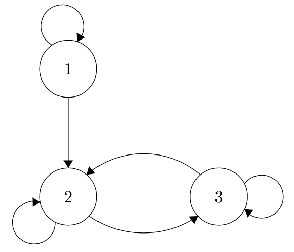
Here, State 1 is transient; if we start in State 1, we might circle back to State 1 for a while, but eventually we’ll go to states 2 and 3 and we will bounce around there for all of time, never returning to 1 (2 and 3 are called a ‘class’; you will learn more about this in a course on stochastic processes). States 2 and 3 are recurrent; if you start in either one, you know you’ll get back eventually.

Recurrence is relatively straightforward, but there are some subtleties. Consider this chain:

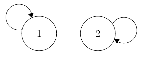
Although it seems a little strange, both States 1 and States 2 are recurrent. You might guess that they are transient, since if we start at State 1, we never get to State 2. The key here, though, is in the definition: a state if recurrent if, given that you start at the state, you have a probability of 1 of returning. Clearly, if you start in 1 or 2, you will definitely return (over and over and over again, until the end of time!).

Concept 10.2: Irreducible vs. Reducible (chain characteristic)

This is sort of like the chain generalization of recurrence and transience (definitions that, recall, apply to individual states). Irreducible chains are chains where it’s possible to go from any state to any other state. It doesn’t matter if that path might take a long time, it just matters that it’s possible. The two chains from the recurrent examples above are both reducible (not irreducible; for the sake of memory, think about how a reducible chain can be reduced into distinct, smaller parts). In both cases, we can’t go from 2 to 1, ever.

If a chain is irreducible, this implies that all states in the chain are recurrent. This is intuitive: if all of the states are somehow connected (irreducible chain), then you are guaranteed to get back to where you started at some point (recurrent states). However, the opposite is not true: knowing that all states are recurrent does not imply that the chain is irreducible. Consider the second example from above, where the two states are self-referencing but completely separate. These are both recurrent but obviously do not connect to each other, so the chain is reducible.

Concept 10.3 Period (state characteristic)

Each state in a Markov Chain has a period. The period is defined as the greatest common denominator of the length of return trips (i.e., number of steps it takes to return), given that you start in that state. This is kind of tricky, so let’s consider an example:

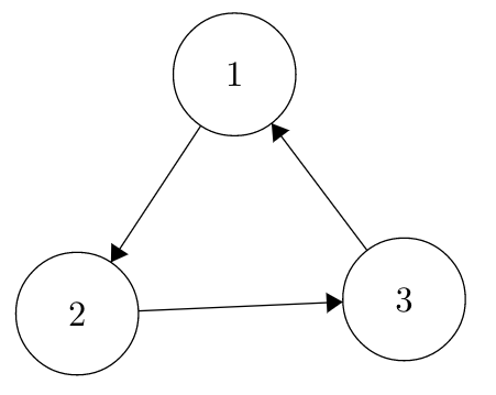
This is a pretty silly chain; we can exactly predict it’s movement over time (that is, it is deterministic). Imagine first that we start in State 1. We know with certainty that in the next step we go to State 2, and then State 3, and then back to State 1. In fact, we know how long every possible path of return to State 1 is: 3 steps, 6 steps, 9 steps, etc. The greatest common denominator of these path lengths is 3, so State 1 (and the other two states) have period 3.

Now let’s add in a slight twist. Consider this chain:

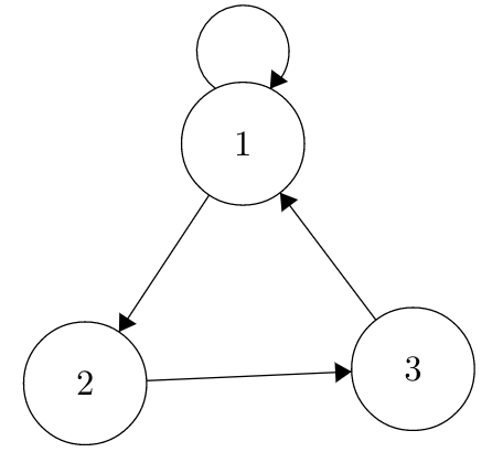
All we did was add a self-referencing edge to State 1. Let’s think about the period of this state now. If we start in State 1, we could automatically just loop back after one period, but we could also go through the whole chain (to State 2, then 3, then 1) in 3 steps. So two possible return lengths are 1 and 3 (there are more, of course), and already the greatest common denominator of these path lengths is 1 So State 1 has period one.

What about State 2? If we start at State 2, we know we will go to State 3 and then State 1. However, there we could stay in State 1 for any period of time before returning to State 2. We could return in 3, 4, 5, etc. number of steps. Again, the greatest common denominator here is 1, so State 2 also has period 1. You can check, but the same holds for State 3.

Concept 10.4: Periodic vs. Aperiodic (chain characteristic)

If all states in a chain have period 1, that chain is aperiodic. Otherwise, it is a periodic chain. The first chain in the previous example (the chain that is entirely deterministic, it goes from 1 to 2 to 3 to 1, etc.) is periodic, the second chain (similar chain but with a self-referencing edge to State 1) is aperiodic.

Concept 10.5: $n$-step Transition Matrix

This is not really a ‘property’ of Markov Chains, but it’s a very important result that we need to discuss. Recall how we write our transition matrix $Q$. We say that $q_{i,j}$, or the $\{i, j^{th}\}$ entry in $Q$ is the transition probability of going from State $i$ to State $j$. For example:

\[\mathbf{Q} = \left[\begin{array} {rr} .4 & .6 \\ .5 & .5 \\ \end{array}\right]\]

This is a chain with 2 states (which we can label 1 and 2). The probability of going from State 1 back to State 1 is .4 (the entry in the first row, first column), the probability from going from State 1 to State 2 is .6 (first row, second column), and State 2 has equal probabilities of going back to State 2 or to State 1 (second row is $(1/2, 1/2)$). This transition matrix gives the probability of moving from state to state in 1-step (that is, going from State 1 to State 2 in a single step). How could we find the probability of going from state to state in multiple steps? For example, if we start at State 1, what is the probability that, after 3 steps, we are at State 2?

This seems like a complicated problem, but the answer boils down quite nicely. A proof that we won’t recreate here shows that $Q^n$, or the transition matrix raised to the power of $n$, gives the $n$-step transition matrix. That is, the $\{i,j^{th}\}$ entry of $Q^n$ gives the probability of going from State $i$ to State $j$ in exactly $n$ steps. To answer our question above (if we start at State 1, what is the probability that we are at State 2 three steps later) we would simply raise our matrix to the power of 3 and look at the entry in the first row and second column.

Thankfully, R is extremely good at creating matrices and performing calculations with them (especially because this book does not assume linear algebra). We can perform the above ‘matrix to a power’ calculation using the matrix command (the nrow argument determines the number of rows, and the ncol argument determines the number of columns; see the R glossary for more). We use %^% to raise matrices to a power. After performing this calculation, we see that entry in question is $.546$, meaning that the probability that we start in State 1, go 3 steps and end up in State 2 is $.546$. Notice that the rows of this matrix still sum to 1; that’s because this is still a valid transition matrix, just generalized to multiple steps (if a row summed to $.8$, for example, we wouldn’t know where the chain went in 3 steps a full 20% of the time!). Also notice that the rows are starting to look similar to each other; more on this in the next section.

#define the matrix
Q = matrix(c(.4, .6,
             .5, .5), nrow = 2, ncol = 2, byrow = TRUE)

#raise the matrix to the power of 3
Q%^%3

##       [,1]  [,2]
## [1,] 0.454 0.546
## [2,] 0.455 0.545

Stationary Distributions

This is probably the trickiest part of our work with Markov Chains. The stationary distribution, which we notate by $s$, can (generally, usually, under certain conditions) be thought of as the long-run distribution of our chain. What does that mean? Well, if we have a Markov Chain, and we let our random particle bounce around for a very long time, then $s$ describes the distribution of the location of the particle. Even more specifically, you can think of $s_1$ as the proportion of time that the particle is in State 1 over the long run, and $s$ codes the proportion of time that the particle is in each of the states (not just State 1). We will formalize this later.

By this notation, then, if we have $m$ states in our chain, $s$ is a 1 by $m$ vector: one row by $m$ columns. The $i^{th}$ value in the vector gives the amount of time that the chain will spend in State $i$. Before even doing any math, we can guess at the stationary distribution of this chain, which we will call the ‘coin’ chain:

As you might have guessed, this chain models the process of randomly flipping a fair, two-sided coin. The states are simply what side the coin shows on the $i^{th}$ flip. Knowing that the stationary distribution is the proportion of time spent in each state, we can guess that $s = (.5,.5)$. That is, we believe that we’re going to spend half of our time in the heads state, and half in the tails state.

This is, of course, a pretty simple example, and things get more difficult as the chains grow more complicated themselves. Now, let’s discuss more properties of the stationary distribution, and how to find it in some simple cases.

In general, the stationary distribution $s$ is given by:

\[sQ = s\]

Where, again, $Q$ is the transition matrix. We know that $s$ is a $1 \;x \;m$ vector and $Q$ is a $m \;x \;m$ matrix (in general, $a \;x \;b$ means a matrix with $a$ rows and $b$ columns), so the multiplication on the left does indeed produce something that is $1 \;x \;m$ on the right (this makes more sense if you are familiar with linear algebra; don’t worry about it too much if you are not). Let’s step through this intuition. We saw earlier that the entries of $Q^m$ give us the probability of traveling from state to state in exactly $m$ steps. What about if we don’t know which state we will start in? That is, what if $X_t$ is random, and we have its distribution (that is, the distribution of where the chain will be at time $t$)? How can we find the distribution of $X_{t + 1}$ (i.e., the distribution of where the chain will be at time $t + 1$)?

When we consider a ‘distribution’ in this setting, we simply just mean the probability that $X_t$ or $X_{t + 1}$ takes on any of the states in the matrix. We can write this as a $1 \; x \; m$ vector; a single row where the $i^{th}$ entry codes the probability of being in the $i^{th}$ state. Let’s call this vector $\theta$. In general, if $\theta$ is the distribution of where the particle lands at $X_t$, then the distribution of where the particle lands at $X_{t + 1}$ is given by:

\[\theta Q\]

Recall that $\theta$ is a $1 \; x \; m$ vector and $Q$ is a $m \; x \; m$ matrix, so this multiplication comes out to a $1 \; x \; m$ vector, which is what we want (we want a distribution over the $m$ states). We’re not going to go over the proof here, but think briefly about why it makes sense. We raise the matrix to a power to find the probability of multiple steps, and here we multiply it by the ‘starting weights’ (i.e., distribution at the current step) to find the distribution for the next step.

Let’s do an example of this. Consider what $\theta$ would be in the ‘coin chain’ example above for $X_1$; i.e., the distribution of where the chain starts. Since we are flipping a fair coin, we are equally likely to start with a heads or tails, meaning $\theta = (1/2, 1/2)$. Therefore, if we want the distribution of $X_2$ (where the coin goes on the next move) we write:

\[\theta Q\]

We just talked about how $\theta = (1/2, 1/2)$, and we know $Q$ is a 2x2 matrix full of $1/2$ (going from any side of the coin to any other side of the coin has probability $1/2$) so we can do this calculation in R. Similar to the power calculation above, we use %*% for matrix multiplication.

#define Q
Q = matrix(c(1/2, 1/2, 
             1/2, 1/2), ncol = 2, nrow = 2)
theta = c(1/2, 1/2)

theta%*%Q

##      [,1] [,2]
## [1,]  0.5  0.5

The output comes to $(1/2, 1/2)$, meaning that the distribution of $X_2$ (if we start $X_1$ at heads or tails with equal probabilities) is $1/2$ heads, and $1/2$ tails. No surprises here.

Anyways, the point here is that if $X_t$ has distribution $\theta$ and $Q$ is the transition matrix, then $\theta Q$ gives the distribution of $X_{t + 1}$. Let’s return, then to the result we saw with stationary distributions: $sQ = s$. This is pretty interesting: if the distribution of $X_t$ is $s$, then this equation shows that the distribution of $X_{t + 1}$ is also $s$. That is, once we get to $s$, we stay in it; the following states also all have this distribution! This is really interesting, and gives credence to the name ‘stationary.’ In fact, in the coin chain we just worked with above, when we used $(1/2, 1/2)$ for $\theta$ and multiplied it by $Q$, we got $(1/2, 1/2)$ back; this shows that $(1/2, 1/2)$ is in fact the stationary distribution, which we guessed at earlier! It also shows that we start in the stationary distribution (this $\theta$ was the distribution of the first flip) so we actually don’t have to wait for convergence to $s$.

Technically speaking, you could always solve $sQ = s$ if you had $Q$, but when you have a large number of states it gets computationally difficult. Since this book does not assume experience with linear algebra, we won’t worry much about it here; it’s just worth mentioning that this is the formula. This tidbit also might be helpful for intuiting how $s$ works (as we discussed, once we are in $s$, we stay there).

Now let’s talk about some of the properties of stationary distributions as they relate to chains in general. For any irreducible Markov Chain (remember, this means that each state is recurrent, or that we can get from any state to any other state) with a finite number of states, we know:

A stationary distribution $s$ exists.
The stationary distribution $s$ is unique.
$s_i = \frac{1}{r_i}$, where $r_i$ is the expected amount of time that it takes to return to State $i$, given that you start at State $i$.

Again, these are more sort of just general facts to know. We’re not going to prove any of them here, but it’s interesting to know that each irreducible MC (Markov Chain) has a unique stationary distribution (and interesting to know that there might not be a unique stationary distribution if this condition doesn’t hold!). The final point is interesting, too (that the long run time we spend in a state is the reciprocal of the average return time of that state). This is intuitive; if it takes a long time to return to a state, then we would expect the amount of time we spend there to be small. This matches the third result above, since if $r_i$ is big then $s_i$ is small. It doesn’t necessarily help us that much in terms of finding the stationary distribution, since $r_i$ can also be difficult to calculate, but it’s an interesting property to remember.

Concept 10.6: Long-run MC Behavior

Recall how we introduced the stationary distribution: a vector that describes the long-run behavior of the chain. Formally, if we have a Markov Chain with stationary distribution $s$, then the distribution of $X_t$ converges to $s$ as $t$ goes to $\infty$ (the only condition is that $Q^n$ is positive in all entries, where $Q$ is the transition matrix and $n$ is a power that we raise it to).

More specifically, if we raise $Q$ to a large enough power (i.e., take enough steps) every row of $Q$ starts to approach the stationary distribution. Does this make sense? Well, we just saw that the MC approaches the stationary distribution, and we know $sQ = s$ (once we are in the stationary distribution, we stay there), so every row of $Q$ should be $s$. Consider the first row: this is a $1 \; x \; m$ vector that codes the probability of going from State 1 to any other state. If we are in the stationary distribution, this should be $s$ (no matter what state we are coming from, since recall that once $X_t$ has the stationary distribution, so does $X_{t + 1}$) so we should see this row (and all other rows) become $s$. Recall the R example from earlier, where we found the 3-step transition matrix of a 2x2 Markov Chain:

#define the matrix
Q = matrix(c(.4, .6,
             .5, .5), nrow = 2, ncol = 2, byrow = TRUE)

#raise the matrix to the power of 3
Q%^%3

##       [,1]  [,2]
## [1,] 0.454 0.546
## [2,] 0.455 0.545

Here, we can already start to see the MC approaching the stationary distribution: already, the rows are extremely similar. If we raise it to a higher power, then we see the two rows equalize:

#define the matrix
Q = matrix(c(.4, .6,
             .5, .5), nrow = 2, ncol = 2, byrow = TRUE)

#raise the matrix to the power of 3
Q%^%10

##           [,1]      [,2]
## [1,] 0.4545455 0.5454545
## [2,] 0.4545455 0.5454545

Here, it looks like the stationary distribution is around $s = (.4545, .5454)$ (it spends 45.45% of time in State 1, and 54.54% of time in State 2 in the long run).

Concept 10.7: Reversibility

This is a chain characteristic; just like chains can be irreducible or aperiodic, they can also be reversible. This concept of reversibility also has a close connection to stationary distributions. We define a chain as reversible if there is a vector $s$ such that:

\[s_i q_{ij} = s_j q_{ji}\]

For all $i,j$ where, as usual, $q_{ij}$ is the probability of going from $i$ to $j$, or the $\{i,j^{th}\}$ entry in the transition matrix $Q$, and $s$ is a row vector of length $m$ (if there are $m$ states in the chain).

If the above holds, then we know that the chain is reversible. Further, if the above holds, we know that $s$ (normalized) is the stationary distribution!

A quick aside; what does ‘normalized’ mean? We just have to make $s$ a vector that sums to 1. So, for the vector $(1,2)$ we would normalize by dividing each entry by the sum of all entries, which is 3, to get $(\frac{1}{3}, \frac{2}{3})$. Now we have a vector of probabilities that sum to 1, which is good because a stationary distribution must sum to 1 (the particle has to be somewhere on the chain. If the stationary distribution summed to .5 for example, we wouldn’t know where the particle was half of the time!).

Anyways, this definition can be difficult to wrap our heads around. Let’s talk through it for a second. What does $s_i q_{ij}$ represent? Well, $s_i$ is the long run fraction of time that we are in State $i$, and $q_{ij}$ is the probability of going from $i$ to $j$. If $s_i q_{ij} = s_j q_{ji}$, you can sort of see how the path between $i$ and $j$ is kind of ‘reversible.’ Think about it as the fraction of time you spend transitioning from $i$ to $j$ (which is the long run probability that you are in $i$, times the probability that you move from $i$ to $j$) being the same as the fraction of time you spend transitioning from $j$ to $i$ (the long run probability you’re in $j$, times the probability of going from $j$ to $i$).

Why do we care about reversibility? Reversible chains are often nicer to work with, and, maybe more importantly, reversibility provides us with a way to find the stationary distribution. Recall the heads/tails Markov Chain; we mentioned what the stationary distribution was, but we’ll take a closer look here. The transition matrix (where we consider the first row and column as heads and the second row and column as tails) is given by:

\[ \mathbf{Q} = \left[\begin{array} {rr} .5 & .5 \\ .5 & .5 \\ \end{array}\right] \]

Is this chain reversible? Remember, to prove reversibility, we must show that for some $s$:

\[s_i q_{ij} = s_j q_{ji}\]

Where $i$ and $j$ can take on the values 1 or 2, since we have a chain with two. Let’s think about finding a vector $s$ that satisfies the above equation. When $i = j$, the above is trivially correct (we get $s_i q_{ii} = s_i q_{ii}$). We only have to prove this, then, when $i \neq j$, or:

\[s_{1} q_{1,2} = s_{2} q_{2, 1}\]

Since $i$ and $j$ can only take on values 1 and 2, this is the only case in which $i$ and $j$ are different.

We know that, from the transition matrix, $q_{1, 2} = q_{2, 1} = .5$. That is, the probability of going from State 1 to 2 and vice versa is .5. Therefore, we can cancel out the $q$ terms on both sides and we are left with:

\[s_{1} = s_{2}\]

Pretend for a moment that we didn’t already find the stationary distribution for the chain; could we construct a stationary distribution that satisfied the above condition? Of course! We write:

\[s \propto (1,1)\]

We use $\propto$ (or ‘proportional to’) since this is not quite a legal stationary distribution; we will momentarily normalize it so that it sums to 1. Anyways, with this $s$, then the reversibility condition:

\[s_i q_{ij} = s_j q_{ji}\]

Holds for all $i$ and $j$.

So, we have proven that this chain is reversible. What else did we find? The stationary distribution! We saw that $s$ is proportional to $(1,1)$, and we have to normalize it so we have a vector of valid probabilities that sum to 1. We do this by dividing each entry but the sum of the vector, 2, to get:

\[s = (\frac{1}{2}, \frac{1}{2})\]

Which matches the intuitive answer we arrived at earlier, and the answer we found from the $sQ = s$ calculation.

Again, the interpretation here is that we spend roughly half of our time in each state, which makes a lot of sense based on the transition matrix. So, this exercise proved that the chain is reversible and also yielded us the stationary distribution. We can confirm that this is the stationary distribution with a simulation in R. We define an empty path X, the transition matrix Q, and generate new values for the path X based on the rows of the transition matrix Q. As the stationary distribution we solved for suggests, we spend amount equal amounts of time in each state.

#replicate
set.seed(110)
sims = 1000

#define the transition matrix
Q = matrix(c(1/2, 1/2, 
             1/2, 1/2), nrow = 2, ncol = 2)

#keep track of X (the stochastic process)
X = rep(NA, sims)

#start at a random spot
X[1] = sample(1:2, 1)

#run the loop
for(i in 2:sims){
  
  #sample according to the transition matrix;
  #   use the row associated with X_{i - 1} 
  #   for the sample probabilities
  X[i] = sample(1:2, 1, prob = Q[X[i - 1], ])
}


#should spend an equal amount of time in each state
table(X)/sims

## X
##     1     2 
## 0.486 0.514

Concept 10.8: Symmetric Transition Matrices

We actually stumbled upon something interesting in this previous example. We saw that, with this coin chain, $q_{ij} = q_{ji}$ for all $i,j$ (this held trivially when $i = j$, but also held when $i \neq j$, since every transition probability was $1/2$). We then saw that, since $q_{ij} = q_{ji}$, the reversibility condition simplified to $s_i = s_j$ for all $i,j$, meaning in essence that every entry of $s$ was the same; that is, $s$ is uniform over the states (each state has the same probability). The $q_{ij} = q_{ji}$ condition also indicates something else: that we have a symmetric transition matrix; that is, the matrix is ‘reflected’ across the diagonal line starting from the top left and moving to the bottom right (it might be easier to visualize the fact that the $\{i,j\}$ entry equals the $\{j,i\}$ for all $i,j$). So, the result that we found is that if an irreducible chain has a transition matrix that is symmetric, the stationary distribution is uniform over the states. That is, we have probability $1/m$, where $m$ is the number of states, at being in each state in the long run.

Example 10.1: Random Walk on Undirected Network

Before moving on to another topic, we’ll discuss an example with a specific type of Markov Chains: the Random Walk on an Undirected Network. Here is an example of this type of chain.

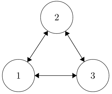
A couple of notes here. Generally, when writing a Random Walk on an Undirected Network, the edges are just drawn as lines without arrows; the arrows here are drawn to emphasize that each edge is a two-way street. For example, you can go from 2 to 1, but also from 1 to 2.

Another observation is that there are not written probabilities that are associated with each edge (that is, we don’t see the probability of going from State 1 to State 2, like in earlier chains). That’s because, for this type of Markov Chain, the edge probabilities are proportional to the number of edges connected to each node. That is, if we’re at node 1, we choose to follow an edge randomly and uniformly. Here, we have two edges, one going to State 2 and one going to State 3, so we would choose one of these edges, each with an equal .5 probability. If a state had $n$ edges, it would pick an edge at random and each edge would have a $\frac{1}{n}$ probability of being picked.

So, in this case, we have edges between all of the three states, and each edge has a .5 probability associated with it (since each state has 2 edges protruding from it). Let’s discuss the characteristics of this chain. It is clearly irreducible: we can get from any state to any other state (pretty quickly, in fact). Since the chain is irreducible, every state is recurrent (if we start at State 1, we will get back there eventually!). What about periodicity? Consider State 1: we can go from State 2 and back to State 1 (so a return trip of length 2) or we can go from State 1 to State 2, then to State 3, then back to State 1 (so a return trip of length 3). Already, our two return trip lengths, 2 and 3, have a GCD of 1, so State 1 is aperiodic (and, by symmetry, the other two states are aperiodic as well; we could apply the same argument to States 2 and 3). That means the entire chain is also aperiodic.

We can also write the transition matrix Q:

\[\mathbf{Q} = \left[\begin{array} {rrr} 0 & .5 & .5 \\ .5 & 0 & .5 \\ .5 & .5 & 0 \\ \end{array}\right]\]

How about the stationary distribution? We could immediately use the property that we just saw: recognize that this is a symmetric transition matrix, meaning that the stationary distribution is uniform across the states. Therefore, in the long run, we have an equal probability of $1/3$ of being in each state.

However, let’s try to find the stationary distribution in the general case of a Random Walk on an Undirected Network (not just this specific case with 3 states that are all connected; in the general case, we don’t necessarily need to have all of the states be directly connected!). We will do this by finding the $s$ vector that satisfies the reversibility condition; by definition, if it does satisfy this condition, then it must be the stationary distribution for the chain. Remember, to show reversibility, we have to prove this strange equation:

\[s_i q_{ij} = s_j q_{ji}\]

For all $i \neq j$ (since, again, this clearly holds when $i = j$: we just get $s_i q_{ii} = s_i q_{ii}$).

Let’s think about the transition probabilities. What are $q_{ij}$ and $q_{ji}$? Well, the probability of going from State $i$ to $j$ is just 1 over the number of nodes connected to $i$ (since we pick among the edges at random and only one is connected to $j$). In this notation, we will call $d_i$ the number of edges attached to node $i$, or the degree of node $i$. So, the probability of going from $i$ to $j$, or $q_{ij}$, is just $\frac{1}{d_i}$. Plugging in for the transition probabilities, we are left with:

\[\frac{s_i}{d_i} = \frac{s_j}{d_j}\]

Can we construct a vector $s$ that satisfies the above? Well, imagine if we let $s_i = d_i$ for all $i$. Then we are left with:

\[\frac{d_i}{d_i} = 1 = 1 = \frac{d_j}{d_j}\]

And the equation is satisfied. So, we showed that for $s \propto (d_1, d_2, ... d_m)$ (again, we write $\propto$, or ‘proportional to,’ since we still have to normalize $s$), if we have $m$ nodes, satisfies the reversibility equation.

What else did we get? You guessed it, the stationary distribution! We have to again normalize our $s$ vector by dividing by the sum of the vector, but this gives…

\[s = (\frac{d_1}{\sum_1^m d_i}, ..., \frac{d_m}{\sum_1^m d_i})\]

…as the stationary distribution, for the general case of a Random Walk on an Undirected Network (we know it must be the stationary distribution because it satisfies the reversibility condition). This is pretty valuable, since for any Markov Chain with this structure, even one with trillions of nodes connected in all sorts of different ways, this result holds. It’s actually pretty intuitive: if State $i$ has many edges connecting to it (a ‘high degree’), then we would expect the random particle to visit it often. In this case, this also means that $d_i$ is large, which means the $i^{th}$ entry in the stationary distribution is large, which means that in the long run we have a relatively high probability of being in State $i$.

We can confirm this result with a simulation in R. We will create a matrix called edges that randomly determines if two states are connected (we will then force the matrix to be symmetric, and ensure that no state is connected to itself. It would be a problem if a full row had no edges to other states, but this is very unlikely and didn’t occur in this specific simulation when we had a large number of states and a 1/2 probability of two random states being connected; recall that we can ‘set a seed’ to replicate random simulations). We then determine the transition matrix Q based on this edges matrix, and simulated the Markov Chain from there (the X[i] value is generated according to the row in Q associated with X[i - 1]). We see that the proportional time spent in each state closely matches the analytical stationary distribution (the degree of a node divided by the sum of degrees). If we increased the number of simulations, the plot would match even more.

#replicate
set.seed(110)
sims = 1000

#define the number of states
m = 10

#create a matrix that keeps track of edges;
#   randomly assign if two states are connected
#   we have to be careful that we don't get a row with no edges;
#   in this case, we are ok
edges = matrix(rbinom(m*m, 1, 1/2), nrow = m, ncol = m)

#force the matrix to be symmetric; edges are two-way streets
edges = forceSymmetric(edges)

#diagonal should be 0; a state isn't connected to itself
diag(edges) = rep(0, m)

#define the transition matrix
Q = edges/rowSums(edges)

#keep track of a path for X
X = rep(NA, sims)

#generate the starting value
X[1] = sample(1:m, 1)

#run the loop
for(i in 2:sims){
  
  #generate a new value, based on the row associated with the previous value
  X[i] = sample(1:m, 1, prob = Q[X[i - 1], ])
}

#proportion of time in each state should match s
plot(table(X)/sims, main = "Stationary Distribution", 
     type = "h", col = "black", lwd = 3, xlab = "State",
     ylab = "Proportion of time in a State", ylim = c(0, .2))
lines(1:m, rowSums(edges)/sum(edges), type = "p", pch = 16,
      col = "firebrick3", lwd = 3)

#make a legend
legend("topright", legend = c("Empirical Time in States", "Analytical Stationary Distribution"),
       lty=c(1,20), lwd=c(2.5,2.5),
       col=c("black", "firebrick3"))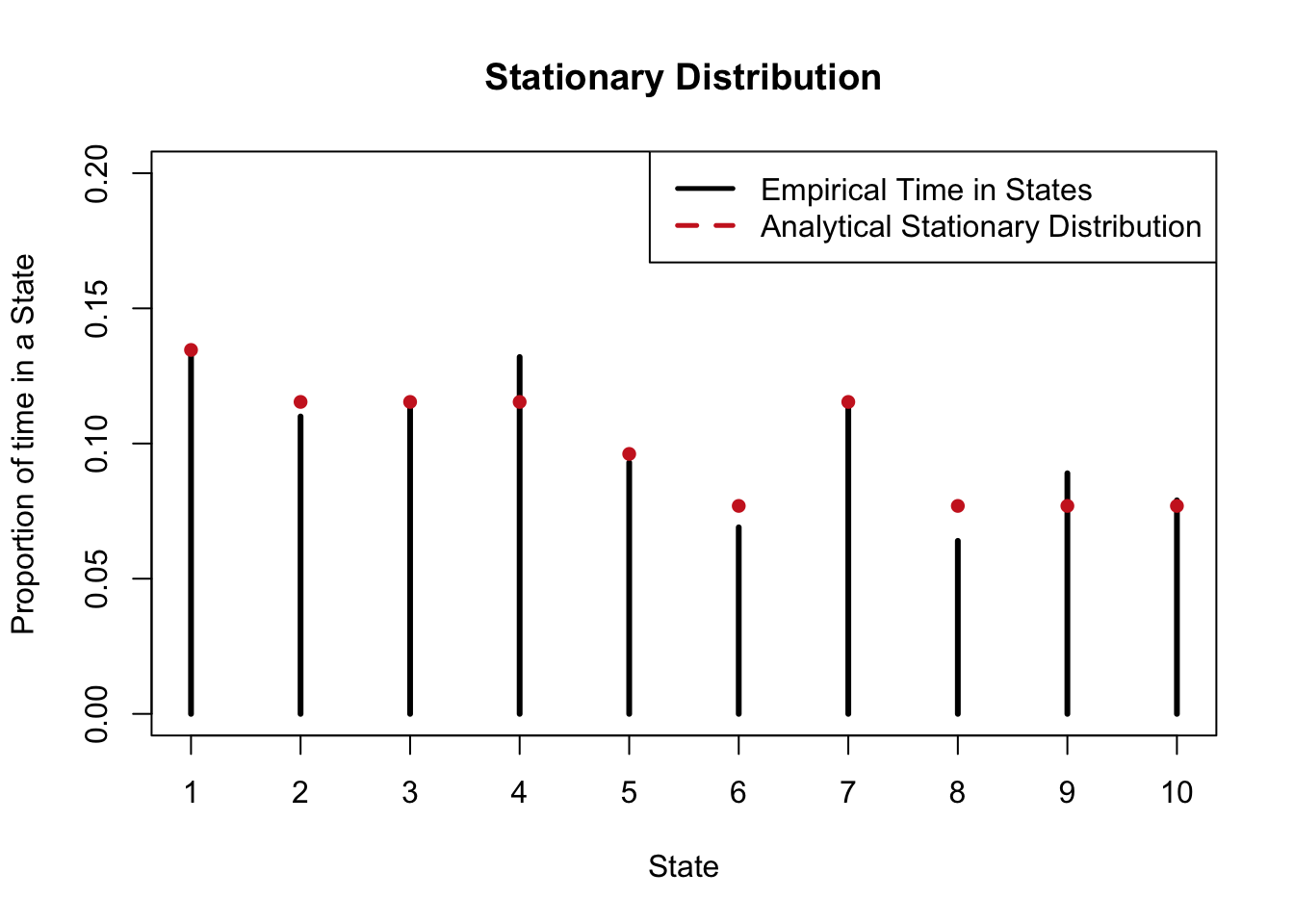

This is really just the tip of the iceberg for Markov Chains and stochastic processes. Be sure to read more about stochastic processes, as they are as interesting as they are useful; the applications range from physics, to biology, to finance, and more. You can explore Markov Chains more with our Shiny App; reference the tutorial video below for more.

Click here to watch this video in your browser. As always, you can download the code for these applications here.

Hidden Markov Models

Before we close the final chapter, let’s discuss an extension of the Markov Chains that begins to transition from Probability to Inferential Statistics.

It’s best to think about Hidden Markov Models (HMM) as processes with two ‘levels.’ There is a Markov Chain (the first level), and each state generates random ‘emissions.’ The key is that the Markov Chain is unobservable and the emissions are observable. This is a bit tricky to wrap your head around. Consider this example with ‘emotions’: define states in the Markov Chain with double circles, and emissions as single circles. The edges, as usual, are notated with the probability that we follow each edge.

Here, we have the ‘emotional states,’ happy and sad, as the Markov Chain, and the ‘reactions,’ smile and frown, as the emissions. Based on the HMM set-up, we say that the emotional states are unobservable, but the reactions are observable. That is, we can see if a person is smiling or frowning, but we cannot observe if they are happy or sad! In this specific example, the probabilities are intuitive: a happy person is more likely to smile than frown (probabilities of $3/4$ and $1/4$), and similarly a sad person is more likely to frown than smile (probabilities of $5/6$ and $1/6$).

From this simple set-up, many complex questions arise. It’s very natural to think about making inferences on (guessing) the true state of the Markov Chain (here, happy or sad) based on the emission that we observe (here, smile or frown). That is, if we see someone smile, what is the probability that they are happy? If we’ve seen someone smile 4 ‘rounds’ in a row, what’s the probability that they are happy? If we see someone smile, what is the probability that they are sad in the next ‘round?’ If we didn’t know the transition probabilities of the emotional states Markov Chain (here, they are defined), could we use the observed emissions to estimate these transition probabilities?

Further, like Markov Chains, these models can complicate very quickly. Imagine a hidden Markov Chain with many states, and each with many different possible emissions. We will try to further wrap our heads around HMMs with a simple example.

Example 10.2: Poisson HMM

Consider this HMM structure:

Again, we imagine that double circles are hidden states, and that regular circles are the emissions. We see that the transition probabilities of the Markov Chain are known: we have probability $1/2$ of transitioning from any state to any other state. In this case, we say that the emissions follow Poisson distributions. If we are in State 1, the emission is a $Pois(a)$ random variable; if we are in State 2, the emission is a $Pois(b)$ random variable, where $a$ and $b$ are known constants. We start in State 1 or State 2 randomly (with equal probabilities).

Given that we observe an emission of 0, what is the probability that we are currently in State 1? Does this result make sense?
Let $X_t$ be the value of the emission at time $t$. Find the PMF of $X_t$.
Find $E(X_t | X_s)$ and $Cov(X_t, X_s)$ for $t > 1$ and $s < t$.
Find $Var(X_t)$.

Analytical Solution:

Define $C$ as the event that we are currently in State 1, and $D$ as the event that we observe an emission of 0. We are interested in $P(C|D)$. Using Bayes’ Rule, we write:

\[P(C|D) = \frac{P(D|C)P(C)}{P(D)}\]

We can expand the $P(D)$ in the denominator using LOTP:

\[= \frac{P(D|C)P(C)}{P(D|C)P(C) + P(D|C^c)P(C^c)}\]

Let’s now break down these probabilities. First, consider $P(C)$, or the marginal probability that we are currently in State 1. This structure is completely symmetric with respect to States 1 and 2: we start in a uniformly random states, and transition between every state with probability $1/2$. Therefore, by symmetry, there must be equal probabilities of being in State 1 or State 2 marginally (that is, unconditionally), so $P(C) = 1/2$, and thus $P(C^c) = 1 - P(C) = 1/2$ (since $P(C^c)$ is just the probability of being in State 2).

Now consider $P(D|C)$, or the probability of observing an emission of 0 if we are in State 1. By the structure of this problem, if we are in State 1, the emission is distributed $Pois(a)$. Therefore, we just need the probability that a $Pois(a)$ random variable takes on the value 0. Recall that if $X \sim Pois(\lambda)$, the PMF of $X$ is defined as:

\[P(X = x) = \frac{e^{-\lambda} \lambda^x}{x!}\]

To find the probability of a $Pois(a)$ random variable taking on the value 0, then, we plug in $a$ for $\lambda$ above (since $a$ is our parameter) and we plug in 0 for $x$ (since we want the probability of the random variable crystallizing to 0). This comes out to $e^{-a}$, so we have that $P(D|C) = e^{-a}$.

Finally, consider $P(D|C^c)$, or the probability of observing an emission of 0 if we are in State 2. This is similar to the calculation above: we need the probability that a $Pois(b)$ random variable (i.e., the emission distribution of State 2) takes on value 2. By the same calculation above, this comes out to $e^{-b}$. Putting it all together:

\[P(C|D)= \frac{P(D|C)P(C)}{P(D|C)P(C) + P(D|C^c)P(C^c)} = \frac{e^{-a}}{e^{-a} + e^{-b}}\] Notice that we dropped the $P(C)$ and $P(C^c)$ terms because they are both $1/2$ and thus cancel out.

Does this result make sense? First, it is bounded between 0 and 1, meaning it returns a valid probability. When will this probability be high? If $a$ is 1 and $b$ is very large, this value will be close to 1, since $e^{-b}$ is very small compared to $e^{-1}$ and thus the numerator and denominator are very close in size. This is intuitive: if $a$ is 1 and $b$ is large and we observe an emission of 0, then we expect that we are in State 1, since it is much more likely to observe a draw of 0 from a $Pois(1)$ random variable (the emission distribution of State 1) than from a Poisson random variable with a very high parameter (the emission distribution of State 2). A similar argument applies if $a$ is very large and $b$ is 1; in this case, the conditional probability of being in State 1 will be small, which makes sense because it is now far more likely that State 2 emits a 0 compared to State 1. In general, when $a$ and $b$ are very different, the probability we solved for will be close to 0 or 1; practically, this makes sense because it means we are working with two very different emission distributions, and thus the actual emission will likely help us discern the underlying distribution with a high probability. If $a$ and $b$ are similar, then the opposite occurs. For example, if $a = b$, the probability comes out to $1/2$: this makes sense because the emission distributions are now symmetric, and thus we’re equally likely to observe a 0 in either state, so the emission does not help us to discern the underlying state at all!

Similarly to the first part of the problem, define $C$ as the event that we are in State 1 at time $t$. Using LOTP, we can expand the PMF of $X_t$:

\[P(X_t = x) = P(X_t = x|C)P(C) + P(X_t = x|C^c)P(C^c)\]

We’ve already seen how $P(C) = P(C^c) = 1/2$. Now, consider $P(X_t = x|C)$. If we are in State 1 at time $t$, then the emission $X_t$ has a $Pois(a)$ distribution (and, similarly, we have a $Pois(b)$ emission distribution if we are in State 2 at time $t$) and we can thus plug in the PMF of a Poisson directly:

\[= \frac{1}{2}\big( \frac{e^{-a} a^x}{x!} + \frac{e^{-b} b^x}{x!}\big)\]

\[= \frac{1}{2} \big(\frac{e^{-a} a^x + e^{-b} b^x}{x!}\big)\]

This is clearly not the PMF of a Poisson (unless we have that $a = b$, and then the above would simplify to the PMF of a $Pois(a)$ random variable), so we cannot say that $X_t$ is Poisson (it’s interesting that this ‘mixture’ of Poissons is not Poisson!). It is intuitive that $X_t$ is not Poisson; imagine if $a$ is very small and $b$ is very large. Half of the time $X_t$ will be taking on small values (when we are in State 1, we have emissions $Pois(a)$, and $a$ is small) and half of the time it will be taking on large values (when we are in State 2, we have emissions $Pois(b)$ and $b$ is small). Therefore, the distribution will have ‘two peaks’ (one near $a$ and one near $b$) which is not a characteristic of a Poisson distribution.

Before we attempt any calculations, consider the relationship between $X_s$ and $X_t$. If we observe $X_s$, or the emission at time $s$, then we essentially can make a guess on what state we are in at time $s$. However, does this inform our prediction for $X_t$ at all? In fact, it does not matter what state we are in at time $s$ (if we are considering $X_t$, the emission at time $t$) since, no matter what state we are in, we move to State 1 or State 2 with equal probabilities in the next step. So, even if $X_s$ gives us information about where we are at time $X_s$, this gives us no information about where we will be at time $t$ (since, every round, the transition is simply a 50/50 draw between the two states, no matter where we start) and thus no information about $X_t$. We can thus say that $X_t$ and $X_s$ are independent.

This allows us to say that $Cov(X_s, X_t) = 0$, since independent random variables have Covariances of 0. It also allows us to drop the conditional in $E(X_t|X_s)$, so we can write $E(X_t|X_s) = E(X_t)$. We can solve this similarly to how we found the PMF of $X$; employing the Law of Total Expectation, and continuing to define $C$ as the event that we are in State 1 at time $t$:

\[E(X_t) = E(X_t|C)P(C) = E(X_t|C^c)P(C^c)\]

We’ve seen that $P(C) = P(C^c) = 1/2$. We also know that $X_t | C \sim Pois(a)$ and $X_t | C^c \sim Pois(b)$, so $E(X_t | C) = a$ and $E(X_t | C^c) = b$. Putting it all together:

\[E(X_t|X_s) = E(X_t) = \frac{a + b}{2}\]

This is quite intuitive: we have a 50/50 chance of a $Pois(a)$ emission vs. a $Pois(b)$ emission, so the overall mean should be the average of the means of these emission distributions ($a$ and $b$).

Recall the definition of Variance:

\[Var(X_t) = E(X_t^2) - \big(E(X_t)\big)^2\]

We already know $E(X_t)$, so the second term is solved. Consider $E(X_t^2)$. We actually solved for the PMF of $X_t$ earlier in this problem, meaning we can use LoTUS to try and solve this expectation:

\[E(X_t^2) = \frac{1}{2} \sum_{x = 0}^{\infty} x^2 ( \frac{e^{-a} a^x}{x!} + \frac{e^{-b} b^x}{x!})\]

We can distribute the $x^2$ and split this into two sums:

\[=\frac{1}{2} \Big( \sum_{x = 0}^{\infty} x^2 \cdot \frac{e^{-a} a^x}{x!} + \sum_{x = 0}^{\infty} x^2 \cdot \frac{e^{-b} b^x}{x!}\Big)\]

It may look like we just complicated the calculation, but realize that each sum is the LoTUS expansion for the second moment of a Poisson random variable. That is, if we have $Y \sim Pois(a)$, then the first sum is the expansion for $E(Y^2)$. We know that, in general, $E(X^2) = Var(X) + \big(E(X)\big)^2$, and we know $Var(X) = E(X) = \lambda$ for a $Pois(\lambda)$ random variable. So, we have the second moment of a $Pois(\lambda)$ random variable is $\lambda + \lambda^2$. Putting it together:

\[E(X_t^2) = \frac{1}{2} \big(a + a^2 + b + b^2\big)\]

Returning to the formula for Variance, and recalling that we solved $E(X_t) = \frac{a + b}{2}$, we write:

\[Var(X_t) = E(X_t^2) - \big(E(X_t)\big)^2\]

\[= \frac{1}{2} \big(a + a^2 + b + b^2\big) - \big(\frac{a + b}{2}\big)^2\]

Empirical Solution:

#replicate
set.seed(110)

#increased number of sims for clearer results
sims = 10000


#define simple parameters
a = 2
b = 10

#keep track of Xt and S, as well as Xs (one behind Xt)
S = rep(NA, sims)
Xt = rep(NA, sims)
Xs = rep(0, sims)


#run the loop
for(i in 1:sims){
  
  
  #flip to see which state we are in
  flip = runif(1)
  
  #state 1
  if(flip <= 1/2){
    
    #mark the state
    S[i] = 1
    
    #generate the emission
    Xt[i] = rpois(1, a)
  }
  
  #state 2
  if(flip > 1/2){
    
    #mark the state
    S[i] = 2
    
    #generate the emission
    Xt[i] = rpois(1, b)
  }
  
  #if it's after the first time, mark the previous value
  if(i > 1){
    Xs[i] = Xt[i - 1]
  }
}

#part a; these should match
exp(-a)/(exp(-a) + exp(-b)); length(S[S == 1 & Xt == 0])/length(Xt[Xt == 0])

## [1] 0.9996646

## [1] 1

#part b; show that the PMFs line up
#calculate the analytical PMF
k = as.numeric(rownames(table(Xt)))
PMF = sapply(k, function(x)
  1/2*(dpois(x, a) + dpois(x, b)))


#plots should line up
#empirical
plot(k, table(Xt)/sims, col = "black", main = "Empirical and Analytical PMF", type = "h",
     xlab = "x", ylab = "P(X = x)", xlim = c(min(k), max(k)), ylim = c(0, 1), lwd = 3)

#analytical
lines(k, PMF, main = "Analytical PMF", ylab = "P(X = x)", xlab = "x", col = "red", pch = 20, ylim = c(0, 1), type = "p", lwd = 3)


legend("topright", legend = c("Empirical PMF", "Analytical PMF"),
       lty=c(1,20), lwd=c(2.5,2.5),
       col=c("black", "red"))

#part c.; should get (a + b)/2 = 6 for each
mean(Xt[Xs == 0]); mean(Xt[Xs == 1]); mean(Xt[Xs == 2])

## [1] 6.209199

## [1] 6.144678

## [1] 5.934317

#part d; these should match
1/2*(a + a^2 + b + b^2) - ((a + b)/2)^2; var(Xt)

## [1] 22

## [1] 21.87291

Hidden Markov Models are an excellent topic to close this book, because they begin to hint at the logical next step in Statistical education: Inference. Throughout this book, we have largely gone in one direction: we are given the distributions of some random phenomena (i.e., $X \sim Bin(3, 1/2)$, $Y \sim Pois(10)$, etc.) and are asked to make guesses about the results of these random outcomes (i.e., $E(X|Y)$, $P(X = x, Y= y)$, etc.). HMMs begin to reverse the direction: given results (i.e., emissions), we are asked to make guesses (inferences) about the hidden distribution (i.e., the Markov State that we don’t get to observe). What state are we actually in? What are the probabilities of transitioning between states? What state are we the most likely to be at in 5 rounds? These are all important questions, and you are ready for the next step!

Practice

Before attempting to solve these problems empirically, note the following shortcut for calculating stationary distributions: for a transition matrix $Q$, take the eigenvectors and eigenvalues of the transpose of $Q$, and the eigenvector that corresponds to the eigenvalue 1 is proportional to the stationary distribution (i.e., must be normalized). This is a result from Blitzstein and Hwang (2014), and we will not discuss it much here because this book does not assume linear algebra. To calculate the eigenvectors of the transpose of $Q$, use the code eigen(t(Q)) in R.

Problems

10.1

You flip a fair, two-sided coin 100 times. Define a ‘run’ as a sequence of coin flips with the same value (heads or tails). for example, the sequence $HTTHH$ has 3 runs: the first $H$, then the $TT$ block, then the $HH$ block.

Let $X$ be the number of runs we observe in $n$ flips. We’ve discussed how to find $E(X)$ using indicators. Now, approximate $E(X)$ for large $n$ by imagining this process as a Markov Chain.

10.2

You are repeatedly rolling a fair, six-sided die. Let $X_n$ be the cumulative sum of the rolls after $n$ rolls (so, if we roll a 2 and then a 5, $X_1 = 2$ and $X_2 = 7$). Find the probability that $X_n$ ever hits 7.

Hint: You may leave your answer as a system of equations. You can quickly solve systems of equations in R with the command $solve(a, b)$, where $a$ is the matrix containing the coefficients of the system, and $b$ is the vector giving the RHS of the system.

10.3

Let $X$ be the Markov Chain with transition matrix given by:

\[\left(\begin{array} {cccccc} q & p & 0 & 0 & 0 & 0\\ 0 & q & p & 0 & 0 & 0\\ 0 & 0 & q & p & 0 & 0\\ 0 & 0 & 0 & q & p & 0\\ 0 & 0 & 0 & 0 & q & p\\ 0 & 0 & 0 & 0 & 0 & 1\\ \end{array}\right)\]

Let this chain start at State 0 (the first state), and let $T$ be the time it takes, in discrete steps, until absorption (i.e., get to State 5). Find the PMF of $T$.

10.4

Consider this Markov Chain:

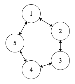
The arrows are not labeled because each arrow has probability $1/2$; that is, there is an equal probability of going clockwise or counterclockwise at every step. Let $T$ be the number of steps it takes to return to State 1. Find $E(T)$ without using facts about the stationary distribution.

10.5

Consider this Markov Chain from the previous problem:

Again, the arrows are not labeled because each arrow has probability $1/2$; that is, there is an equal probability of going clockwise or counterclockwise at every step. Let $T$ be the number of steps it takes to return to State 1. Find $E(T)$ by using facts about the stationary distribution.

10.6

Let $X \sim Pois(\lambda)$. Imagine a Markov Chain with $X + 1$ states and transition matrix $Q$ such that $q_{i, i + 1} = p$ and $q_{i, i} = 1 - p$ for $i = 0, 1, ..., x$ and $q_{x + 1, x + 1} = 1$. Let $M_t$ be the value of the chain (the current state) at time $t$, and let $M_0 = 0$ (start at 0). Find the PMF of $M_X$.

10.7

Consider this Markov Chain, where $a$ and $b$ are valid probabilities.

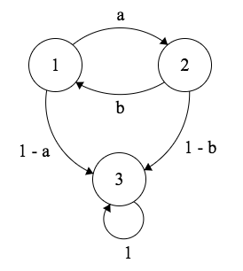
Let $T$ be the time of absorption (time of arrival at State 3). Imagine that we start at State 1.

If $a = b = 1/2$, find $E(T)$.
If $a \neq b$, find $E(T)$.

10.8

Are the following process, $X_t$, Markovian? That is, do they satisfy the Markov property?

Imagine a “branching process” with offspring distribution $Pois(\lambda)$, where $\lambda$ is known. That is, at generation 0, there is 1 individual who has $Pois(\lambda)$ offspring in his lifetime, and each of his descendants independently has $Pois(\lambda)$ offspring. Let $X_t$ be the size of the $t^{th}$ generation.
You repeatedly roll a fair die. Let $X_t$ be the value of the $t^{th}$ roll.
You repeatedly roll a fair die. Let $X_t$ be the mean of roll 1, roll 2, up to roll $t - 1$.
Let $X_t = X_{t - 1} + \epsilon_t$ where $X_0 = 0$ and $\epsilon_i \sim N(0, \sigma^2)$, where $\sigma^2$ is known.
Same as part d., but $\sigma^2$ is unknown.

10.9

Demren is performing a simple, symmetric random walk on the integers; that is, at every integer, he either goes up 1 integer (i.e., 5 to 6) or down 1 integer (i.e., 1 to 0). Let $Y_t$ be his location at time $t$. He starts at 0 at time 1, so $Y_1 = 0$.

We can plot a sample path to show what this process looks like. The x-axis is $t$, or the number of rounds, and the y-axis is $Y_t$, or Demren’s location at time $t$.

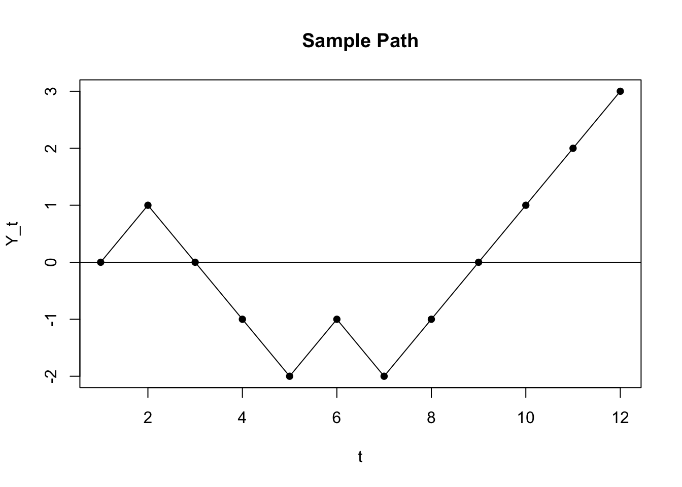
Is $Y_t$ a Markovian process? That is, does it have the Markov property?
Find $P(Y_{2t + 1} > 0)$. You may leave your answer as a sum.

10.10

Find $P(Y_{2t} < 0 \cap max(Y_1, Y_2, ..., Y_{2t}) > 3)$, i.e. the probability that the path hits 3 and ends below 0. You may leave your answer as a sum.

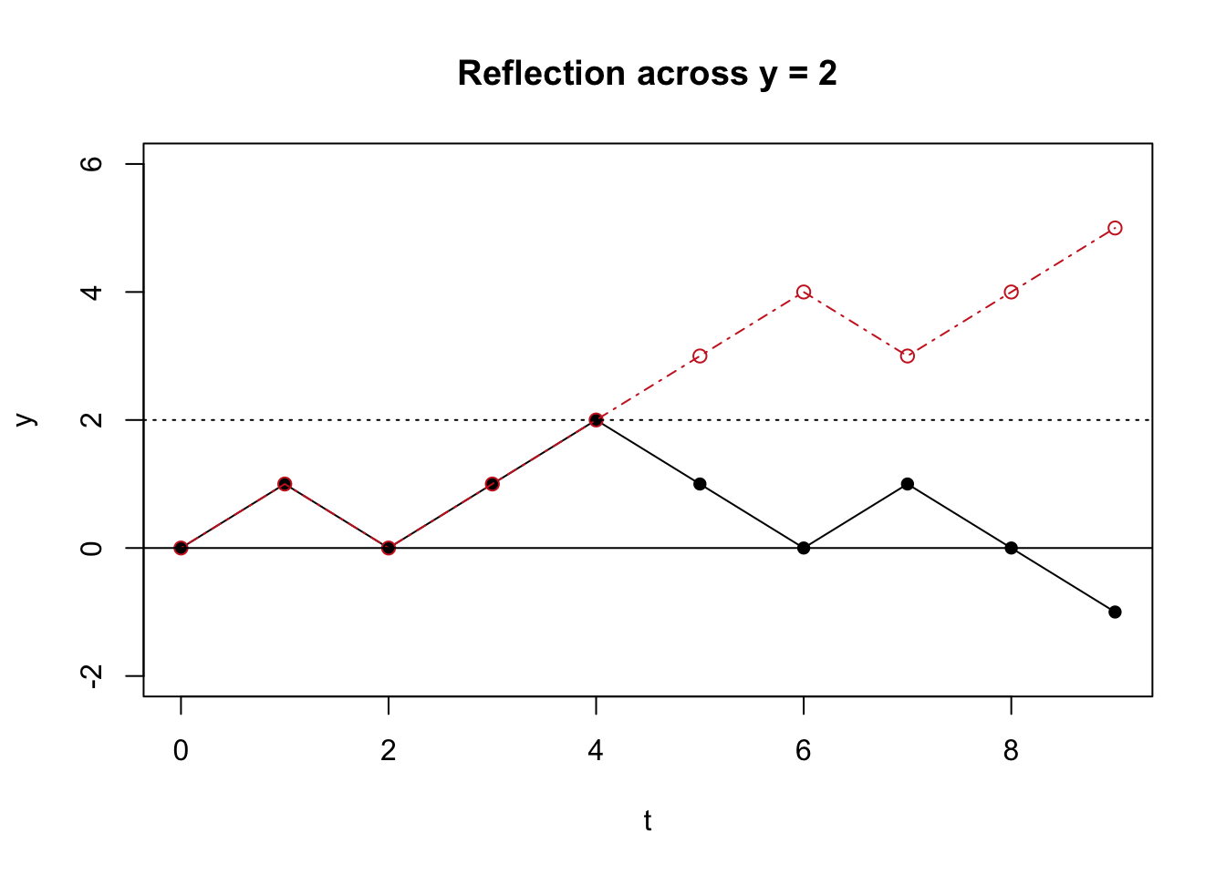
Hint: the ‘reflection principle,’ which applies to this random walk, states that reflecting a path about a horizontal line (i.e., mimicking a path up until some time $t$, and then reflecting a path for the rest of the time interval) creates a path that has the same probability as the original path. Consider the visual below: the original path is in black and the reflected path is in red. The reflected path mimics the original path up until the time that the original path hits a value of 2, and then for the rest of the interval, the reflected path ‘reflects’ the original path across the horizontal line $y = 2$. The reflection principle states that the probability of these two paths are the same.

10.11

A particle is traveling randomly around the vertices of a square. If can only move across vertices connected by edges in one step (i.e., from the bottom left, it can travel to the top left or bottom right, but not the top right). If the particle starts in the top left vertex, what is the probability that it visits the bottom right vertex before it visits the bottom left vertex?

10.12

Consider these two Markov Chains (an $\alpha$ chain and a $\beta$ chain).

Count the number of recurrent states and the number of aperiodic states in each chain, then indicate if the chains are irreducible.

BH Problems

The problems in this section are taken from Blitzstein and Hwang (2014). The questions are reproduced here, and the analytical solutions are freely available online. Here, we will only consider empirical solutions: answers/approximations to these problems using simulations in R.

The problems below often reference Markov Chains that are not reproduced here; see the analytical solutions, linked above, to view these diagrams.

BH 11.2

Let $X_0,X_1,X_2, ...$ be an irreducible Markov chain with state space $\{1,2,..., M\}$, $M \geq 3$, transition matrix $Q=(q_{ij})$, and stationary distribution $\mathbf{s}=(s_1,...,s_M)$. Let the initial state $X_0$ follow the stationary distribution, i.e., $P(X_0 = i) = s_i$.

On average, how many of $X_0,X_1, \dots, X_9$ equal $3$? (In terms of $\mathbf{s}$; simplify.)
Let $Y_n = (X_n-1)(X_n-2)$. For $M=3$, find an example of $Q$ (the transition matrix for the original chain $X_0,X_1, ...$) where $Y_0,Y_1, ...$ is Markov, and another example of $Q$ where $Y_0,Y_1, ...$ is not Markov. In your examples, make $q_{ii}>0$ for at least one $i$ and make sure it is possible to get from any state to any other state eventually.

BH 11.4

Consider the Markov chain shown below, where $0 < p < 1$ and the labels on the arrows indicate transition probabilities.

Write down the transition matrix $Q$ for this chain.
Find the stationary distribution of the chain.
What is the limit of $Q^n$ as $n \to \infty$?

BH 11.5

Consider the Markov chain shown below, with state space $\{1,2,3,4\}$ and the labels on the arrows indicate transition probabilities.

Write down the transition matrix $Q$ for this chain.
Which states (if any) are recurrent? Which states (if any) are transient?
Find two different stationary distributions for the chain.

BH 11.6

Daenerys has three dragons: Drogon, Rhaegal, and Viserion. Each dragon independently explores the world in search of tasty morsels. Let $X_n, Y_n, Z_n$ be the locations at time $n$ of Drogon, Rhaegal, Viserion respectively, where time is assumed to be discrete and the number of possible locations is a finite number $M$. Their paths $X_0,X_1,X_2,...$; $Y_0,Y_1,Y_2,...$; and $Z_0,Z_1,Z_2,...$ are independent Markov chains with the same stationary distribution $\mathbf{s}$. Each dragon starts out at a random location generated according to the stationary distribution.

Let state $0$ be home (so $s_0$ is the stationary probability of the home state). Find the expected number of times that Drogon is at home, up to time $24$, i.e., the expected number of how many of $X_0,X_1,...,X_{24}$ are state 0 (in terms of $s_0$).
If we want to track all 3 dragons simultaneously, we need to consider the vector of positions, $(X_n,Y_n,Z_n)$. There are $M^3$ possible values for this vector; assume that each is assigned a number from $1$ to $M^3$, e.g., if $M=2$ we could encode the states $(0,0,0), (0,0,1), (0,1,0), ..., (1,1,1)$ as $1,2,3, ..., 8$ respectively. Let $W_n$ be the number between $1$ and $M^3$ representing $(X_n,Y_n,Z_n)$. Determine whether $W_0,W_1, ...$ is a Markov chain.
Given that all 3 dragons start at home at time $0$, find the expected time it will take for all 3 to be at home again at the same time.

BH 11.7

A Markov chain $X_0,X_1, ...$ with state space $\{-3,-2,-1,0,1,2,3\}$ proceeds as follows. The chain starts at $X_0=0$. If $X_n$ is not an endpoint ($-3$ or $3$), then $X_{n+1}$ is $X_n-1$ or $X_n+1$, each with probability $1/2$. Otherwise, the chain gets reflected off the endpoint, i.e., from $3$ it always goes to $2$ and from $-3$ it always goes to $-2$. A diagram of the chain is shown below.

Is $|X_0|,|X_1|,|X_2|, ...$ also a Markov chain? Explain.
Let sgn be the sign function: $sgn(x)= 1$ if $x>0$, $sgn(x) = -1$ if $x<0$, and $sgn(0)=0$. Is $sgn(X_0),sgn(X_1),sgn(X_2),\dots$ a Markov chain? Explain.
Find the stationary distribution of the chain $X_0,X_1,X_2,\dots$.
Find a simple way to modify some of the transition probabilities $q_{ij}$ for $i \in \{-3,3\}$ to make the stationary distribution of the modified chain uniform over the states.

BH 11.8

Let $G$ be an undirected network with nodes labeled $1,2,...,M$ (edges from a node to itself are not allowed), where $M \geq 2$ and random walk on this network is irreducible. Let $d_j$ be the degree of node $j$ for each $j$. Create a Markov chain on the state space $1,2,...,M$, with transitions as follows. From state $i$, generate a proposal $j$ by choosing a uniformly random $j$ such that there is an edge between $i$ and $j$ in $G$; then go to $j$ with probability $\min(d_i/d_j,1)$, and stay at $i$ otherwise.

Find the transition probability $q_{ij}$ from $i$ to $j$ for this chain, for all states $i,j$.
Find the stationary distribution of this chain.

BH 11.9

Consider a Markov chain on the state space $\{1,2,...,7\}$ with the states arranged in a “circle” as shown below, and transitions given by moving one step clockwise or counterclockwise with equal probabilities. For example, from state 6, the chain moves to state 7 or state 5 with probability $1/2$ each; from state 7, the chain moves to state 1 or state 6 with probability $1/2$ each. The chain starts at state 1.
Find the stationary distribution of this chain.
Consider a new chain obtained by “unfolding the circle.” Now the states are arranged as shown below. From state 1 the chain always goes to state 2, and from state 7 the chain always goes to state 6. Find the new stationary distribution.

BH 11.10

Let $X_n$ be the price of a certain stock at the start of the $n$th day, and assume that $X_0, X_1, X_2, ...$ follows a Markov chain with transition matrix $Q$. (Assume for simplicity that the stock price can never go below 0 or above a certain upper bound, and that it is always rounded to the nearest dollar.)

A lazy investor only looks at the stock once a year, observing the values on days $0, 365, 2 \cdot 365, 3 \cdot 365, \dots$. So the investor observes $Y_0, Y_1, \dots,$ where $Y_n$ is the price after $n$ years (which is $365n$ days; you can ignore leap years). Is $Y_0,Y_1, \dots$ also a Markov chain? Explain why or why not; if so, what is its transition matrix?
The stock price is always an integer between $0 and $28. From each day to the next, the stock goes up or down by $1 or $2, all with equal probabilities (except for days when the stock is at or near a boundary, i.e., at $0, $1, $27, or $28).

If the stock is at $0, it goes up to $1 or $2 on the next day (after receiving government bailout money). If the stock is at $28, it goes down to $27 or $26 the next day. If the stock is at $1, it either goes up to $2 or $3, or down to $0 (with equal probabilities); similarly, if the stock is at $27 it either goes up to $28, or down to $26 or $25. Find the stationary distribution of the chain.

BH 11.11

In chess, the king can move one square at a time in any direction (horizontally, vertically, or diagonally).

For example, in the diagram, from the current position the king can move to any of 8 possible squares. A king is wandering around on an otherwise empty $8 \times 8$ chessboard, where for each move all possibilities are equally likely. Find the stationary distribution of this chain (of course, don’t list out a vector of length 64 explicitly! Classify the 64 squares into types and say what the stationary probability is for a square of each type).

BH 11.13

Find the stationary distribution of the Markov chain shown below, without using matrices. The number above each arrow is the corresponding transition probability.

BH 11.17

A cat and a mouse move independently back and forth between two rooms. At each time step, the cat moves from the current room to the other room with probability 0.8. Starting from room 1, the mouse moves to room 2 with probability 0.3 (and remains otherwise). Starting from room 2, the mouse moves to room 1 with probability 0.6 (and remains otherwise).

Find the stationary distributions of the cat chain and of the mouse chain.
Note that there are 4 possible (cat, mouse) states: both in room 1, cat in room 1 and mouse in room 2, cat in room 2 and mouse in room 1, and both in room 2. Number these cases $1,2,3,4$, respectively, and let $Z_n$ be the number representing the (cat, mouse) state at time $n$. Is $Z_0,Z_1,Z_2,...$ a Markov chain?
Now suppose that the cat will eat the mouse if they are in the same room. We wish to know the expected time (number of steps taken) until the cat eats the mouse for two initial configurations: when the cat starts in room 1 and the mouse starts in room 2, and vice versa. Set up a system of two linear equations in two unknowns whose solution is the desired values.

References

Blitzstein, J. K., and J. Hwang. 2014. Introduction to Probability. Chapman & Hall/CRC Texts in Statistical Science. CRC Press. https://books.google.com/books?id=z2POBQAAQBAJ.

Chapter 10 Markov Chains

Motivation

Introduction to Markov Chains

Characteristics of Markov Chains

Concept 10.1: Recurrent vs. Transient (state characteristic)

Concept 10.2: Irreducible vs. Reducible (chain characteristic)

Concept 10.3 Period (state characteristic)

Concept 10.4: Periodic vs. Aperiodic (chain characteristic)

Concept 10.5: \(n\)-step Transition Matrix

Stationary Distributions

Concept 10.6: Long-run MC Behavior

Concept 10.7: Reversibility

Concept 10.8: Symmetric Transition Matrices

Example 10.1: Random Walk on Undirected Network

Hidden Markov Models

Example 10.2: Poisson HMM

Practice

Problems

10.1

10.2

10.3

10.4

10.5

10.6

10.7

10.8

10.9

10.10

10.11

10.12

BH Problems

BH 11.2

BH 11.4

BH 11.5

BH 11.6

BH 11.7

BH 11.8

BH 11.9

BH 11.10

BH 11.11

BH 11.13

BH 11.17

References