Chapter 7 Covariance and Correlation

“I used to think correlation implied causation. Then I took a Statistics class; now I don’t.”

“Sounds like the class helped!”

“Well, maybe.”

Adapted from this comic from xkcd.

We are currently in the process of editing Probability! and welcome your input. If you see any typos, potential edits or changes in this Chapter, please note them here.

Motivation

We continue our foray into Joint Distributions with topics central to Statistics: Covariance and Correlation. These ‘two brothers,’ as we affectionately refer to them, will allow us to quantify the relationships between multiple random variables and will give us the tools to tackle novel, higher-dimensional problems. These are among the most applicable of the concepts in this book; Correlation is so popular that you have likely come across it in a wide variety of disciplines. We’ll also step further into working with multiple random variables and discuss Transformations and Convolutions (distributions of the sums of distributions).

Covariance

The first ‘brother’ is likely the less popular of the two, mostly because he is widely less applicable. However, he’s also the oldest; it’s important to talk about him first because we will eventually define Correlation in terms of Covariance.

Let’s start with a qualitative framework; you can probably already guess what Covariance ‘essentially means.’ We know that variance measures the spread of a random variable, so Covariance measures how two random random variables vary together. Unlike Variance, which is non-negative, Covariance can be negative or positive (or zero, of course). A positive value of Covariance means that two random variables tend to vary in the same direction, a negative value means that they vary in opposite directions, and a 0 means that they don’t vary together. If two random variables are independent, their Covariance is 0, which makes sense because they don’t affect each other and thus don’t vary together (this relation doesn’t necessarily hold in the opposite direction, though, which we will see later on).

This might seem a little confusing, so let’s actually define Covariance and continue from there. For two random variables \(X\) and \(Y\), you can define the Covariance \(Cov(X,Y)\) as:

\[Cov(X,Y) = E\Big(\big(X-E(X)\big)\big(Y - E(Y)\big)\Big)\]

So, in words, the expected value of the product of the random variables minus their respective means. Recall that \(X\) and \(Y\) are random variables, while \(E(X)\) and \(E(Y)\) are averages and thus are constants.

Now that we can actually see this definition, let’s think about what positive and negative Covariances mean. Let’s say that \(X\) and \(Y\) tend to vary together; specifically, \(X\) tends to be large (i.e., above it’s mean) when \(Y\) is also large. We already said that if two things vary together, we should get a positive Covariance, and let’s see if this holds when we plug in to the formula. Well, when \(X\) crystallizes to a value above its mean, \(X-E(X)\) will be positive, and if \(Y\) crystallizes to a value above it’s mean when \(X\) is large/above its mean, then \(Y-E(Y)\) is also positive. Multiplying two positives together yields a positive Covariance, which ultimately matches our intuition. Of course, Covariance would also be positive if both \(X\) and \(Y\) tended to vary below their means; we would just be multiplying a negative by a negative to get a positive value.

Think about a negative Covariance, then. This occurs when (in this simplified framework of thinking) one random variable tends to be above its mean and the other tends to be below its mean; you would be multiplying a negative by a positive (or a positive by a negative) to yield an overall negative Covariance.

Hopefully the gist of Covariance is now clear. The biggest problem with this metric in practice is how arbitrary the units are. For example, we could measure something in inches (perhaps the vertical leap heights of two NBA basketball teams) and get a Covariance of, say, 12.4. Then we could convert the inch measurements to centimeters (still the exact same jumps, just in different units) and my Covariance would change because of the unit change. The point is that the actual magnitude of Covariance is arbitrary (it depends on the units) and not that helpful for intuition. You’ve likely experienced this with variance thus far; i.e., what does a variance of 100 dollars really mean? This is a big limitation of Covariance, and it is key to remember that really the most informative part about the metric is the sign. Sure, Covariance can tell you when two things vary together (Covariance is positive) but it’s hard to tell how strong that relationship is based on the actual magnitude of the Covariance (Correlation will supplement this, of course, by providing valuable information on strength).

Anyways, Covariance shows up quite a lot in Statistics, especially in problems that require an understanding of certain specific properties of Covariance. Let’s dive deeper into some of these properties of Covariance now. Everything we do can be derived from what we’ve already written down about Covariance, and even if we don’t prove it here, it’s really just easy algebra to prove it for yourself.

First, you’ll probably notice that our definition of Covariance seems very similar to the definition of Variance. Recall that for a random variable \(X\):

\[Var(X) = \Big(E\big(X - E(X)\big)^2\Big)\]

In fact, let’s go a step further and find the Covariance of \(X\) against itself, or \(Cov(X,X)\), by plugging into the definition of Covariance:

\[Cov(X,X) = E\Big(\big(X-E(X)\big)\big(X - E(X)\big)\Big) = \Big(E\big(X - E(X)\big)^2\Big)\]

And voila, we’ve arrived back at the Variance! So, a key property of Covariance is that \(Cov(X,X) = Var(X)\), as we’ve just shown here.

Now let’s look at properties that have to do with the Covariance of two different random variables. We’ll start simple:

\[Cov(X,Y) = Cov(Y,X)\]

This makes sense, because really the only difference is flipping the order of the product in the definition of Covariance from above, which of course gives the same thing, since \(a \cdot b = b \cdot a\).

Another fruitful property that we recover after considering the expectation expansion of Covariance is:

\[Cov(X,Y) = E(XY) - E(X)E(Y)\]

Again, this can be found simply by multiplying out the original definition of Covariance. In fact, let’s try deriving this for practice. We start with the definition of Covariance from above, and multiply out:

\[Cov(X,Y) = E\Big(\big(X-E(X)\big)\big(X - E(Y)\big)\Big)\] \[= E\Big(XY - YE(X) - E(X)Y + E(X)E(Y)\Big)\]

Now we take the outer expectation. Recall that \(E(X)\) is a constant (we are taking an average), and the expectation of a constant is just a constant itself (so \(E(c) = c\) for any constant \(c\)). Applying this, we get:

\[= E(XY) - E(Y)E(X) - E(Y)E(X) + E(Y)E(X)\] \[= E(XY) - E(X)E(Y)\]

As we said above.

This is an interesting result because (recall from previous chapters) if \(X\) and \(Y\) are independent random variables, then \(E(XY) = E(X)E(Y)\), and thus the above expression simplifies to 0. This makes sense, because remember that if \(X\) and \(Y\) are independent then their Covariances are 0. In general, how would we calculate \(Cov(X, Y)\) if \(X\) and \(Y\) are dependent? We could find \(E(X)\) and \(E(Y)\) the usual way, and then use a 2-D LoTUS calculation to find \(E(XY)\).

Next, remember how the Variance of a constant is 0, since constants don’t vary at all? Covariance has a similar property. Specifically:

\[Cov(X,c)=0\]

For any constant \(c\). This is intuitive, because \(c\) doesn’t vary at all and thus \(X\) doesn’t vary with it. Algebraically, if you return to the original definition of Covariance and plug in the constant \(c\) to this algebraic definition, you’ll see that you end up multiplying by \(c - E(c) = c - c = 0\), which of course makes the entire expression go to 0.

Now, we will dive a little deeper. This next property will eventually allow us to deal with the Variance of a sum of multiple random variables (where these random variables are not necessarily independent; in previous chapters, we have only worked with the independent case). This can be derived, again, by simply plugging into the definition of Covariance. For random variables \(X\), \(Y\) and \(Z\):

\[Cov(X,Y+Z) = Cov(X,Y) + Cov(X,Z)\]

Again, to prove this, you would simple have to plug in \(Y+Z\) wherever you see a \(Y\) in the original formula for Covariance and multiply out. Eventually, you would get to the above result, which is extremely valuable. The quick way to remember it is that everything on the left side of the comma has a Covariance with everything on the right side of the comma; to find the Covariance between the two sides, we need to write the Covariance of \(X\) with \(Y\), and of \(X\) with \(Z\). If we had \(X + Z\) on the left side of the comma and \(Y\) on the right side of the comma, then we would have to add the Covariance of \(X\) with \(Y\) to the Covariance of \(Z\) with \(Y\). In general, we essentially draw a line between every element on the left to every element on the right, and add a Covariance for each pair.

This ‘sum within a Covariance’ principle generalizes to the following result:

\[Cov(\sum_{i=1} X_i, \sum_{j=1} Y_j) = \sum_{i,j}Cov(X_i,Y_j)\]

Again, the structure behind this formula is drawing a line between every element on the left (all of the \(X\)’s) and every element on the right (all of the \(Y\)’s). To get the Covariance of the sum of \(X\)’s with the sum of \(Y\)’s, you need the Covariance of every \(X\) with every \(Y\) (\(X_1\) with \(Y_{10}\), \(X_7\) with \(Y_5\), etc.).

This result finally gives us the tools to deal with a sum of Variances, which is a concept that has eluded us for some time now. Let’s first consider \(Var(X+Y)\). We can re-write this in terms of Covariance; recall how \(Cov(X,X) = Var(X)\), so \(Var(X + Y)\) can also be written as \(Cov(X+Y,X+Y)\), or the Covariance of \(X + Y\) with itself.

Why expand the Variance like this? It seems like we’re just complicating things. Well, remember the rule that when taking the Covariance of sums, we draw a line from every element on the left of the comma to every element on the right of the comma and add Covariance of all of these pairs. If we want to take the Covariance of \(X+Y\) with itself, \(X+Y\), we need the Covariance of \(X\) with \(X\), the Covariance of \(Y\) with \(Y\), and the Covariance of \(X\) with \(Y\) (twice, since you can draw a line from the first \(X\) to the second \(Y\) and a line from the first \(Y\) to the second \(X\)). This comes out to:

\[Cov(X+Y,X+Y) = Cov(X,X) + Cov(Y,Y) + 2Cov(X,Y)\]

We know \(Cov(X,Y) + Cov(Y, X) = 2Cov(X,Y)\) because \(Cov(X,Y) = Cov(Y, X)\), as we saw earlier. And, of course, we know that the Covariance of something with itself is just its variance, so we can further simplify this expression:

\[Var(X+Y) = Cov(X + Y, X + Y) = Var(X) + Var(Y) + 2Cov(X,Y)\]

Let’s think about this term on the right for a bit. You might have seen it at the AP Statistics level. We can think of \(X\) and \(Y\) as the returns of two stocks (both stocks have a return, which is basically how much money they’re expected to make, and both have risks, which measure how much the return fluctuates; this is an example that Mike Parzen, from the Harvard Statistics Department, often uses in his courses to build intuition). In the Statistics ‘world,’ it’s pretty much the norm to think of return as the average, or expectation, of a stock, and risk as the variance. So, say that you were building a portfolio (a compilation of multiple stocks) and wanted to find the risk and return of the entire portfolio (in this case, just two stocks, \(A\) and \(B\), which we will treat as random variables). It wouldn’t be hard to find the return, or the expectation of the portfolio: we know that expectation is linear, so \(E(A+B) = E(A) + E(B)\). This is a result we’ve used a lot before, but until now we would not have been able to find \(Var(A + B)\). We know now that it is the sum of the two individual variances plus two times the Covariance of \(A\) and \(B\) together.

We could break this down into the ‘individual risks’ of the stocks - the separate Variances \(Var(A)\) and \(Var(B)\) - and the ‘interactive’ risks of them together - the Covariance term \(2Cov(A,B)\). The individual risk is straightforward enough (just the marginal variance of each stock), but think more about the interactive risks. If two stocks tend to move together, then they are certainly riskier; if one plummets, then the other has a greater chance of plummeting (it’s sort of the ‘putting all of your eggs in one basket’ strategy vs. the ‘diversification’ argument). Well, we know that if two stocks move together, then their Covariance will be positive, which of course means that we are adding a positive value to our overall measure of variance for the entire portfolio. So, in a nutshell, when we look for the variance of a sum of two different random variables, we need the individual variances and then the ‘interactive’ variance (here, the Covariance term) to get the overall variance.

It’s also worthwhile to note that if two random variables are independent and thus their Covariance is 0, then the variance of their sum is just the sum of their variances (the last term - the Covariance - is 0 because the random variables are independent). We’ve used this result before but have not proven it, and now you can really see why this holds true (the extra Covariance term goes away).

Finally, consider the relationship between ‘independence’ and a ‘Covariance of 0.’ We’ve said that if random variables are independent, then they have a Covariance of 0; however, the reverse is not necessarily true. That is, if two random variables have a Covariance of 0, that does not necessarily imply that they are independent. The reason for this frustrating result is that Covariance, in a manner of speaking, measures linear independence. Two random variables might have a quadratic relationship, and this relationship would be ‘detected’ by the Covariance calculation. For example, if we have two random variables \(X\) and \(Y\) such that \(X = Y^2\), then \(X\) and \(Y\) are clearly not independent. Knowing \(Y\) tells us exactly what \(X\) is (i.e., if \(Y = -2\), we know \(X = 4\)), and knowing \(X\) narrows \(Y\) down to two possible values (unless \(X = 0\), since \(Y\) must then also be 0). However, they would have a Covariance of 0 because their relationship is not linear. This is an important distinction to remember because it is easy to automatically apply, but not necessarily true in all cases.

We can confirm this strange result in R by creating a vector x that takes on the integers from -10 to 10 and a vector y that squares all of the values in the x vector. Clearly, these are very dependent (think of x as the support of a random variable \(X\). If \(X\) crystallizes to 4, then we know \(Y\), or the random variable associated with the y vector, must be 16). However, despite being dependent, they have a Covariance of 0 (so, a Covariance of 0 does not imply independence).

#define x and y = x^2
x = -10:10
y = x^2

#plot x and y; clearly a relationship
plot(x, y, pch = 16)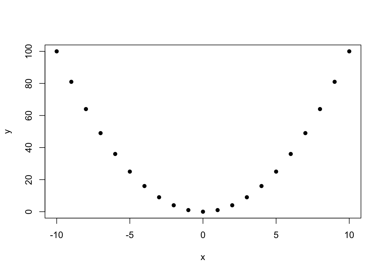

#should get a Covariance of 0
cov(x, y)

## [1] 0

Correlation

This second, younger ‘brother’ is probably a little more useful, and you will see him more often in real life situations. The reason that we cover Correlation second is that we define it in terms of Covariance (i.e., Covariance is the ‘older’ brother). Specifically, our mathematical definition is as follows for random variables \(X\) and \(Y\):

\[\rho = Corr(X,Y) = \frac{Cov(X,Y)}{\sigma(x)\sigma(y)}\]

Here, we use the \(\sigma(x)\) to mean “Standard Deviation of \(X\).” We also included the \(\rho\) (the Greek letter ‘rho’) because that’s often the notation most often used for Correlation.

So, Correlation is the Covariance divided by the standard deviations of the two random variables. Of course, you could solve for Covariance in terms of the Correlation; we would just have the Correlation times the product of the Standard Deviations of the two random variables. Consider the Correlation of a random variable with a constant. We know, by definition, that a constant has 0 variance (again, for example, the constant 3 is always 3), which means it also has a standard deviation of 0 (standard deviation is the square root of variance). So, if we tried to solve for the Correlation between a constant and a random variable, we would be dividing by 0 in the calculation, and we get something that is undefined. This is actually kind of logical, because it doesn’t make sense to think about a constant value being correlated with something.

In this book, we won’t be going through nearly as many properties with Correlation as with Covariance, but there are important characteristics that we need to discuss. First of all, the most important part of Correlation is that it is bounded between -1 and 1.

What exactly does this interval mean? The idea here is as the Correlation grows in magnitude (away from 0 in either direction) it means that the two variables have a stronger and stronger relationship. Like the Covariance, the sign of the Correlation indicates the direction of the relationship: positive means that random variables move together, negative means that random variables move in different directions. Let’s look at the extreme points. The endpoints, -1 and 1, indicate that there is a perfect relationship between the two variables. For example, the relationship between feet and inches is always that 12 inches equals 1 foot. If you plotted this relationship, it would be an exactly perfect line; the two variables relate to each other totally and completely in this fashion (of course, feet only equals inches scaled to a specific factor - here, the factor is 12 - but the relationship is still a perfect mapping). Therefore, the Correlation is 1. Obviously, this is pretty rare, if not non-existent, in real life data, since two random phenomena don’t usually map to each other by a constant factor. We can check that this ‘feet-inches’ relation holds in R:

#define a vector of inches
inches = 1:20

#convert to feet
feet = inches*12

#should get 1
cor(feet, inches)

## [1] 1

Now consider the other extreme on the bounds of Correlation. A Correlation of 0 means that there is no linear relationship between the two variables. We already know that if two random variables are independent, the Covariance is 0. We can see that if we plug in 0 for the Covariance to the equation for Correlation, we will get a 0 for the Correlation. Therefore, again, independence (in terms of random variables) implies a Correlation of 0. However, again, the reverse is not necessarily true. Since, again, Covariance and Correlation only ‘detect’ linear relationships, two random variables might be related but have a Correlation of 0. A prime example, again, is \(x = y^2\) (recall that we showed in R that the Covariance is 0, which means the Correlation must also be 0).

Anyways, and we won’t deal with this much here (we mainly have a theoretical focus), but a good rule of thumb for Correlation is that a value of \(\rho\) (remember, the notation we use for Correlation) between .4 and .6 is a moderate relationship, between .6 and .8 is a strong relationship, and above .8 is a very strong relationship (in absolute value; remember that a negative Correlation just means that the two random variables vary inversely). Just as a quick note, you might see artificially high Correlations (.8 and above) intended to prove a point in your classes, but be assured that in the real world Correlations are generally much smaller. Anyways, these topics will come up in discussions with more applied tilts.

Here, then, we have the first reason that we may prefer Correlation to Covariance: it not only gives us the direction of the relationship (do the random variables move together or in opposite ways/is the Correlation positive or negative) but the strength of the relationship (depending on how large the Correlation is in absolute value). Remember that with the Covariance scales arbitrarily, so we can never be sure how strong a Covariance is by looking at the magnitude.

This is a nice segue into the next reason why we prefer Correlation: it is unitless, which is exactly why we can rely on the magnitude to inform us as to the strength of the relationship. If we consider the formula for Correlation, we’re pretty much taking the variance of two variables together and dividing out by the standard deviation of each. This serves to cancel units, and we are left with a value (Correlation) that does not change when units change! Basically, this means that the relationship between inches and feet will stay the same if we are considering the relationship between 3 inches and 3 feet (multiplied by three), not just inches and feet in general. We will always have that nice -1 to 1 interval for \(\rho\), regardless of what units we are working with. We’re essentially standardizing the Covariance. We can confirm in R again that scaling the feet and inches by a constant does not change the fact that Correlation is 1.

#define a vector of inches
inches = 1:20

#convert to feet
feet = inches*12

#scale inches and feet by 3
inches = 3*inches
feet = 3*feet

#should get 1
cor(feet, inches)

## [1] 1

Finally, although this is not necessarily a concept central to this book, it would be irresponsible to talk about Correlation without also talking about causation. Causation, of course, means that changes in one variable cause a change in another variable. If \(T\) was the temperature outside and \(S\) was the amount of sweat someone produced while running, then you could say an increase in \(T\) causes an increase in \(S\) (there is enough scientific evidence to support the fact that hotter temperatures in the environment cause more sweating).

Unfortunately, as you have likely heard from your high school science classes, Correlation alone cannot make that strong a claim. That is, a high Correlation between two random variables indicates that the two are associated, but that their relationship is not necessarily causal in nature. Here’s an example: if you consider the population of adults in the USA, the variables ‘amount of hair on head’ and ‘presence of arthritis in fingers’ are negatively correlated: as one goes down, the other tends to go up (they are going in different directions, so the Correlation is negative). However, that is not to say that a ‘lack of hair’ is causing arthritis, or that head hair someone protects from arthritis. There is clearly a ‘lurking’ variable, age, that is causing both to happen; there is no actual causal link between the correlated variables.

Still confused? Another classic example is considering the Correlation between number of old-fashioned pirates (i.e., old-timey, Blackbeard style) in the world and Global Temperatures. They are very strongly negatively correlated: while the number of swashbucklers has decreased and dwindled over the years, global temperatures are on the climb. However, that’s not because high temperatures caused the decline of pirates (or that pirates fought tooth and nail to keep the global temperature cool); it’s very clear that there are many other factors that played a role in these phenomena and even though they are associated they did not cause each other (like time, and the course of human history!).

The only way to prove causality is with controlled experiments, where we eliminate outside variables and isolate the effects of the two variables in question. The point (and, again, this is not a primary area of concern in this predominantly theoretical book) is to not jump to conclusions when we observe two random variables with high Correlations.

Transformations

We’ve dealt with transformations of random variables for a while now. Usually, we apply LoTUS when we see a transformation (both single and multidimensional), which we use to find the expectation of a function of a random variable (or, a random variable transformed). However, now we will be interested in not just finding the expectation of the transformation of a random variable, but the distribution of the transformation of a random variable.

Earlier in the book, we saw one of the fundamental properties of random variables: that a function of a random variable is still a random variable (if you square a random number, you’re still technically generating a random number!). This is intuitive if you consider a random variable in the official sense: a mapping of some experiment to the real line. A function of this random variable, then, is just a function of the mapping, and essentially a new mapping to the real line, or a new random variable! Therefore, it is reasonable to try and find the ‘distribution’ of a transformed random variable; after all, when we work with a transformation of a random variable, we are still working with a random variable, which has a distribution (remember, the random variable is the meal, and the distribution is the recipe!).

Let’s formalize this. Say that \(X\) is a continuous random variable and that \(Y\) is a function of \(X\) such that \(Y = g(X)\) (remember, this function could be something simple like \(Y = 2X\) or \(Y = X + 4\). The \(g(X)\) is what we plug into LoTUS to get the expectation). Intuitively, \(Y\) is a transformation of \(X\), and thus we are interested in the distribution of \(Y\). If \(g(X)\) is a strictly increasing and differentiable function, we can in fact find the PDF of \(Y\) as follows:

\[f(y) = f(x) \frac{dx}{dy}\]

Where \(f(y)\) is the PDF of \(Y\), \(f(x)\) is the PDF of \(x\), and \(\frac{dx}{dy}\) is the derivative of \(X\) in terms of \(Y\). Also, everything on the right side of the equals sign should be written in terms of \(Y\), which makes sense because we are looking for the PDF of \(Y\).

This formula can seem a little confusing at first, just because of all of the different notation. It’s good to take a step back and think about what we are doing. We have a random variable \(X\) with a known distribution (maybe it’s Exponential, Normal, whatever) and then a random variable \(Y\) that is some transformation of \(X\) (again, a simple example would be \(2X\)). We want to find the PDF of \(Y\). We can break this calculation down into two steps:

We take the PDF of \(X\), or \(f(x)\) in the equation, and we write it in terms of \(Y\). What does it mean to write the PDF in terms of \(Y\)? Well, if the original transformation was \(2X = Y\), then we solve for \(X\) to get \(\frac{Y}{2} = X\), and thus plug in \(\frac{y}{2}\) every time we see an \(x\) in \(f(x)\) (recall that \(f(x)\) is a function of \(x\)).
We take the derivative of \(X\) with respect to \(Y\). That doesn’t sound like it makes a lot of sense, but again, we go back to our transformation \(2X = Y\) and solve for \(X\) to get \(\frac{Y}{2} = X\). Now, we can derive \(X\) with respect to \(Y\). since both sides equal \(X\), just derive the left side with respect to \(Y\); this means we are literally are deriving \(X\) with respect to \(Y\), since \(\frac{Y}{2}\) is \(X\). Anyways, we take that derivative, which is here just \(\frac{1}{2}\), and multiply by the PDF we got in Part 1.

That’s all! These may feel a bit long-winded; it’s just that this formula can be very confusing the first time you see it, and it really helps to break it down into manageable chunks. Let’s do an actual example so that we can really hammer home the structure of these Transformation problems.

Consider the fact that we cited earlier in the book: linear combinations of Normal random variables are still Normal random variables, and the sums of Normal random variables are still Normal random variables. Thanks to our knowledge of Expectation and Variance, we are able to find the Expected Value and Variance of linearly transformed Normals, but we’ve never proved that the resulting distribution is in fact Normal. Now, armed with our knowledge of transformations, we can explore this concept a bit more and provide the proof for a fact that we took for granted earlier.

The problem statement is simple: let \(X \sim N(\mu, \sigma^2)\), and \(\frac{X-\mu}{\sigma} = Z\). Find the distribution of \(Z\).

As we showed in an earlier chapter, subtracting the mean from a Normal random variable and dividing by the standard deviation yields the Standard Normal (again, according to the fact we cited earlier, the linear transformation is still Normal, and we can calculate the mean and variance, which come out to be 0 and 1). However, let’s now prove this result using transformations.

We know that we are looking for the PDF of \(Z\), and just by the formula we know we can find it with:

\[f(z) = f(x)\frac{dx}{dz}\]

Ok, so the first step is to take the PDF of \(X\) and write it in terms of \(Z\); this will give us the \(f(x)\) in the formula above. We know the PDF of a Normal by now, so we write:

\[f(x) = \frac{1}{\sigma\sqrt{2\pi}}e^{-\frac{(x-\mu)^2}{2\sigma^2}}\]

But, based on our steps, we need to replace all of the \(x\)’s with \(z\)’s. Solving \(\frac{X-\mu}{\sigma} = Z\) for \(X\) yields \(X = \sigma Z + \mu\). We can thus plug in \(\sigma z + \mu\) every time we see \(x\) in the PDF, and simplify:

\[ \frac{1}{\sigma\sqrt{2\pi}}e^{-\frac{(\sigma z + \mu -\mu)^2}{2\sigma^2}} = \frac{1}{\sigma\sqrt{2\pi}}e^{-\frac{z^2}{2}}\]

This is starting to look more and more recognizable. Now we have to do the second part in the algorithm from earlier: finding the \(\frac{dx}{dz}\) in the formula above. Again, we solve for \(X\) in the equation with \(Z\) to get \(X = \sigma Z + \mu\). We are looking for the derivative of \(X\) in terms of \(Z\), so we derive the right side of the equation in terms of \(Z\). This gives us \(\sigma\). Now, we can multiply this term by the first part:

\[ \frac{\sigma}{\sigma\sqrt{2\pi}}e^{-\frac{z^2}{2}} = \frac{1}{\sqrt{2\pi}}e^{-\frac{z^2}{2}}\]

Volia! Incredibly, we have gotten to the PDF of a Standard Normal distribution, thus rigorously proving that the distribution of \(Z\) is indeed Normal.

So, remember that even if transformations look complicated, you can break the calculation down into two steps: plugging into the PDF, and then taking a derivative.

One more important point regarding transformations: sometimes finding \(\frac{dx}{dy}\) is challenging. It could in fact be easier to find it’s counterpart: \(\frac{dy}{dx}\). Fortunately, there is a simple formula that relates the two: \(\frac{dx}{dy} = (\frac{dy}{dx})^{-1}\). For example, if \(e^X=Y\) and we need to find \(\frac{dx}{dy}\), we could solve for \(X\) and then take the derivative of the \(Y\) side. This yields \(X = ln(Y)\), and then deriving yields \(\frac{1}{y}\). However, we could also just find \(\frac{dy}{dx}\); this calculation would derive the original in terms of \(X\), which gives \(e^x\), and then take the inverse. We are left with \(\frac{1}{e^x}\). However, we still want our final answer to be in terms of \(Y\), so we have to plug \(Y\) back in. Since we know that \(Y = e^X\), we simply plug in to get \(\frac{1}{y}\), which is the same answer we got from the other method.

The point here is that one derivative will often be easier to find than the other. Don’t do unnecessary work if you don’t have to; use the fact that we can easily convert between the two derivatives.

Finally, let’s extend this concept (as we’ve been doing with many concepts of late) to multiple dimensions. Imagine that we have a vector of Random Variables, \(\vec{X} = (X_1,X_2,...,X_n)\), and a ‘transformed vector’ \(\vec{Y} = g(\vec{X})\). The same formula applies, but in a higher dimensional case.

\[f( \; \vec{y}) = f( \; \vec{x}) \big|\frac{d\vec{x}}{d\vec{y}}\big|\]

The key here is that \(f(\vec{y})\) represents the joint PDF of all of the random variables that make up the vector \(\vec{Y}\), and the same with \(f(\vec{x})\) (it is the joint PDF of the \(X\) vector). The other major difference is the \(\big|\frac{d\vec{x}}{d\vec{y}}\big|\), which looks slightly different from what we had before. In fact, it is quite different; this represents taking the absolute value of the determinant of something called the Jacobian Matrix.

The Jacobian Matrix is essentially the matrix of all possible partial derivatives. For example, if both vectors \(\vec{X}\) and \(\vec{Y}\) were made up of two random variables each (\(X_1,X_2\) and \(Y_1,Y_2\)) then the Jacobian \(\frac{d\vec{x}}{d\vec{y}}\) would be:

\[ \left( \begin{array}{cc} \frac{\partial x_1}{\partial y_1} & \frac{\partial x_1}{\partial y_2} \\ \frac{\partial x_2}{\partial y_1} & \frac{\partial x_2}{\partial y_2}\end{array} \right)\]

A good way to think about this matrix is that the \(x\)’s change as we move vertically and the \(y\)’s change as we move horizontally.

Still confused? We can consider and example. Say that \(X\) and \(Y\) both have two components such that \(X_1 = 2Y_1\) and \(X_2^2 = Y_2\). Find the Jacobian Matrix.

We really can just calculate derivatives and plug in. Recall the trick for finding the derivative of \(X\) in terms of \(Y\): solve for \(X\) and take the derivative of the other side in terms of \(Y\). Putting it together:

\[ \left( \begin{array}{cc} 2 & 0 \\ 0& \frac{1}{2\sqrt{y}}\end{array} \right)\]

This is our Jacobian Matrix. In this example, we only have a 2x2 matrix here, but we could extend this to higher dimensions if we had more random variables.

Of course, recall that for the actual transformation we need to find the absolute value of the ‘determinant’ of the Jacobian. Since this isn’t a book on linear algebra, we won’t really be discussing what a ‘determinant’ is. In fact, most of the time you will only have to find determinants for 2 or 3 dimensional matrices, which have tractable formulas for them. The point is, when we work with determinants, we will refer to simple formulas. In general, for a 2x2 matrix:

\[ \left( \begin{array}{cc} a & b \\ c& d \end{array} \right)\]

The determinant is given by \(ad - bc\). So, in our case, the absolute value of the determinant is just \(\frac{1}{\sqrt{y}}\).

Finally, just like with one-dimensional transformations where we can leverage the trick of flipping the derivative to make our lives easier, the same trick applies to finding the Jacobian. Specifically, \(\big|\frac{d\vec{x}}{d\vec{y}}\big| = \big|\frac{d\vec{y}}{d\vec{x}}\big|^{-1}\). Again, this could make our lives easier if deriving one way is easier than the other way.

Multi-dimensional transformations can be tricky; we do an example in Chapter 8 (the Bank-Post Office result) after we learn about two more important distributions.

Convolutions

Now, we’ll discuss Convolutions. This is a topic similar to Transformations, although with nuanced differences.

The idea here is that with Transformations we were concerned with finding the distribution of a transformed random variable. With Convolutions, we are more interested in finding the distribution of a sum of random variables. When we have seen these in the past (sums of random variables, that is) we’ve usually been able to invoke some Story or MGF to determine the distribution of this new random variable. However, this might not always be the case, and that’s why we need to formalize Convolutions here: to adapt to problems in a more general setting.

Specifically, let’s say that we have two independent random variables \(X\) and \(Y\), and that we want to find the distribution of \(Z\), where \(Z\) is the sum of \(X\) and \(Y\). Knowing that \(X + Y = Z\), we can find the PMF (if the random variables are discrete) as follows:

\[P(Z=z) = \sum_x P(X=x)P(Y=z-x)\]

Let’s consider this formula for a moment: we know that \(X + Y = Z\), so if we fix the \(X\) value to be \(x\), then we know that \(y = z - x\). We then sum up over all possible values of \(x\), and we get our PMF for \(Z\).

The continuous case is very similar. If \(X\), \(Y\) and \(Z\) are continuous:

\[f(z) = \int_{-\infty}^{\infty} f_x(x) f_y(z - x) dx\]

Where \(f_y(z - x)\) is the PDF of \(Y\) evaluated at \(z - x\). Again, this is similar to the discrete case above. While we won’t discuss this much more here, it’s important to be comfortable with these formulas, as they come in handy when dealing with a summation of random variables (especially in situations where MGFs, Stories or other, simpler results don’t apply).

MVN

Now that we understand Covariance and Correlation, we can explore a new multivariate, continuous distribution: the Multivariate Normal (recall that we’ve already learned about the Multinomial, which is a multivariate discrete distribution). This is essentially a Normal distribution in higher dimensions, where we code these ‘higher dimensions’ into a vector. Formally, consider a vector of random variables \((X_1, X_2,...,X_n)\). Now consider some linear combination of this vector: \(Y = c_1X_1 + c_2X_2 + ... + c_n X_n\). If, for any choice of the constants \((c_1, c_2, ..., c_n)\), \(Y\) is Normally distributed, then we say that the vector of random variables is Multivariate Normal.

It can be difficult to wrap your head around this definition the first time that you see it. First, consider a simple example: let \(X \sim N(5, 2)\) and, independently, \(Y \sim N(-1, 3)\). Now imagine the vector \((X, Y)\). This is Multivariate Normal (in this case, since we have two random variables in the vector, we say it is Bi-Variate Normal); imagine writing out a linear combination:

\[c_1 X + c_2 Y\]

We know that linear combinations of Normal random variables are still Normally distributed, so \(c_1 X\) is still Normal, as is \(c_2 Y\). We then know that the sum of independent Normal random variables is still Normal, so we add these two Normal random variables and are left with a Normal. It might appear that \(c_1 = c_2 = 0\) breaks this condition, because plugging in \(c_1 = c_2 = 0\) just yields 0. However, we can consider 0 to be a Normal random variable, with distribution \(N(0, 0)\) (centered around 0, with no variance). This is a certainly a degenerate case, but it is a legitimate Normal distribution nonetheless.

Of course, if the random variables in the vector are not Normal (perhaps \(X\) above had a Poisson, or Exponential, distribution) then the linear combination would not be Normal. However, we might think: “well, as long as the random variables in the vector are Normal, then the vector overall must be Multivariate Normal.” After all, it seems pretty difficult to come up with a linear combination of Normal random variables that is not Normal, especially since we allow for that degenerate \(N(0, 0)\) case (which, in general, allows us to say that any constant technically has a Normal distribution). It’s actually good practice to try and dream up a case where we have a vector of Normal random variables, but a linear combination of these random variables is not Normally distributed. It’s pretty difficult to think of an example, although not impossible: we know that the sum of independent Normal random variables is Normally distributed, but it is possible to create this case we are discussing if the random variables are dependent.

Let’s try to construct one of these strange cases. Let \(X\) and \(Y\) be i.i.d. \(N(0, 1)\) random variables, and let \(Z\) be a random variable that equals \(X\) with probability .99 and \(Y\) with probability .01 (that is, \(X\) and \(Y\) crystallize to values \(x\) and \(y\), and \(Z\) takes on either \(x\) or \(y\) with probabilities .99 and .01). What is the distribution of \(Z\)? Well, 99% of the time it takes on the value of a Standard Normal, and 1% of the time it takes on a value from a…Standard Normal. Since \(Z\) is always taking on Standard Normal values, it is Standard Normal!

Now, is the vector \((X, Y, Z)\) Multivariate Normal? More specifically, is there a choice of constant \(c_1, c_2, c_3\) such that \(c_1X + c_2Y + c_3Z\) is not Normal? Imagine \(c_1 = 1\), \(c_3 = -1\) and \(c_2 = 0\) so that we are left with \(X - Z\). Is this Normal? Let’s think about what this value will be. Most of the time (99% of the time, specifically) we will have \(Z\) crystallize to \(X\), meaning that \(X - Z\) simplifies to 0. The other 1% of the time, we will have \(Z\) crystallize to \(Y\), meaning that we are left with \(X - Y\). What distribution does \(X - Y\) have? Well, \(-Y\) has the same distribution as \(Y\), since multiplying \(Y\) by -1 is the same as flipping it about 0; since the distribution is centered around 0, this is the same as doing nothing! So, you can think of \(X - Y\) as the summation of two independent Standard Normals, which we know to be Normal and specifically is distributed \(N(0, 2)\) (we get the expectation \(E(X - Y) = 0\) and

\[Var(X - Y) = Var(X) + Var(Y) - 2Cov(X, Y) = Var(X) + Var(Y) = 2\].

The Covariance is 0 because the random variables are independent).

So, either \(X - Z\) crystallizes to 0 (99% of the time) or a value from a \(N(0, 2)\) (just 1% of the time). Is this Normally distributed? It doesn’t seem so. How can we think about this more critically? Well, let’s think about the distribution of \(X - Z\) if it were Normal. It would have mean 0 (since \(E(X - Z) = E(X) - E(Z) = 0\)) and variance 1 (we get:

\[Var(X - Z) = Var(X) + Var(Z) - 2Cov(X, Z) = 1 + 1 - 1 = 1\]

We don’t have the tools to solve this Covariance yet, and we will do this example in a later chapter; simply take it for granted for now). So, if \(X - Z\) were Normal, it would have to be the Standard Normal (since it has mean and variance of 0 and 1). Clearly, the random variable we described above (99% of the tie it takes on 0, and 1% of the time a value from \(N(0, 2)\)) is not Standard Normal. We know that the Standard Normal does not take on 0 even close to 99% of the time; in fact, a continuous random variable takes on any specific value with probability 0. It also has far less variance than a Standard Normal (it’s nearly always 0) and we could even shrink this variance further by allowing \(Z\) to take on \(X\) with probability .999, or an even more extreme probability.

Anyways, this linear combination of Normal random variables is not Normal, meaning that \(X, Y\) and \(Z\) are not Multivariate Normal, despite each one being marginally Normal. We can confirm our results in R by generating \(X,Y\) and \(Z\) according to this paradigm. The plots show that each is Standard Normal marginally, but that \(X - Z\) is not Normal.

#replicate
set.seed(110)
sims = 1000

#generate the r.v.'s
X = rnorm(sims)
Y = rnorm(sims)

#set a path for Z
Z = rep(NA, sims)

#run a loop to calculate Z
for(i in 1:sims){
  
  #flip to see if Z takes on X or Y
  flip = runif(1)
  
  #Z takes on X
  if(flip <= .99){
    Z[i] = X[i]
  }
  
  #Z takes on Y
  if(flip > .99){
    Z[i] = Y[i]
  }
}

#set 2x2 graphing grid
par(mfrow = c(2,2))

#plot 4 histograms
hist(X, main = "X", col = rgb(1, 0, 0, 1/4), xlab = "")
hist(Y, main = "Y", col = rgb(0, 1, 0, 1/4), xlab = "")
hist(Z, main = "Z", col = rgb(0, 0, 1, 1/4), xlab = "")
hist(rnorm(sims), main = "N(0, 1)", col = "gray", xlab = "")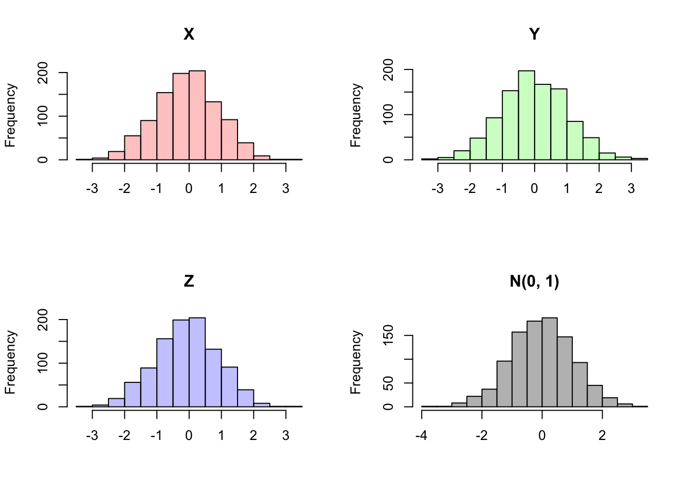

#set 1x2 graphing grid
par(mfrow = c(1,2))

#histograms do not match
hist(X - Z, main = "X - Z", col = rgb(1, 0, 1, 1/4),
     xlab = "")
hist(rnorm(sims), main = "N(0, 1)", col = "gray",
     xlab = "")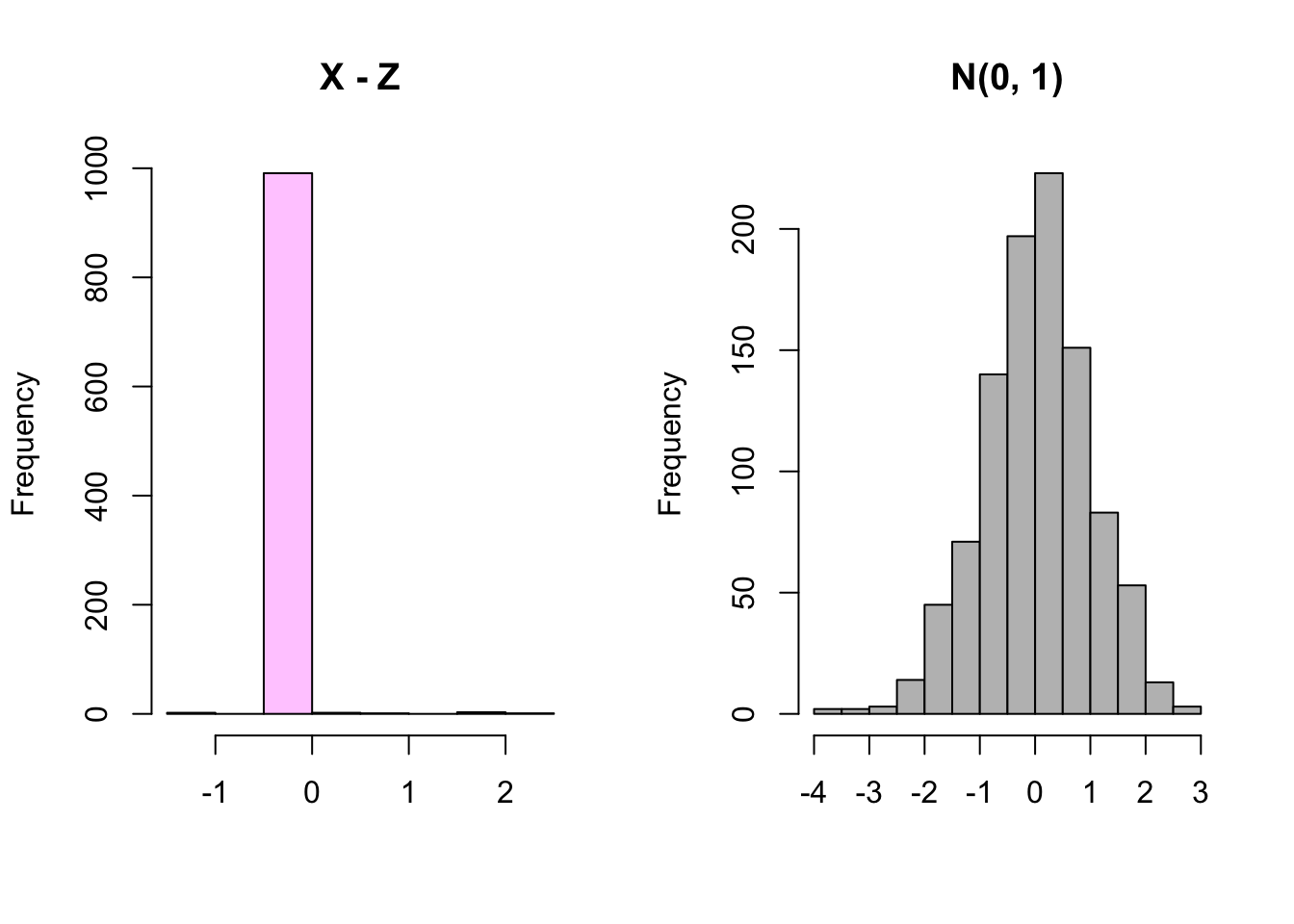

#re-set grid
par(mfrow = c(1,1))

Now, let’s consider a special case of the Multivariate normal, when we have a vector of length 2: this is called a Bivariate Normal. If \(X\) and \(Y\) are Bivariate Normal, we write:

\[(X, Y), \sim BVN\Big( \begin{bmatrix} \alpha \\ \beta \\ \end{bmatrix}, \begin{bmatrix} \sigma_x^2 & \rho \sigma_x \sigma_y \\ \rho \sigma_x \sigma_y & \sigma_y^2 \\ \end{bmatrix}\Big)\]

This notation simply means that \(X \sim N(\alpha, \sigma_x^2)\) and \(Y \sim N(\beta, \sigma_y^2)\) (these are the marginal distributions of \(X\) and \(Y\)), and \(\rho = Corr(X, Y)\). Recall that \(Corr(X,Y) = \frac{Cov(X,Y)}{\sigma_x \sigma_y}\), which we can also write as \(Cor(X, Y) \sigma_x \sigma_y = Cov(X, Y)\), so when we write \(\rho \sigma_x \sigma_y\) above, we are writing the Covariance.

You can think of, then, the 2x1 matrix

\[\begin{bmatrix} \alpha \\ \beta \\ \end{bmatrix}\]

as the mean matrix (it contains information on the marginal means for the random variables) and the matrix \[\begin{bmatrix} \sigma_x^2 & \rho \sigma_x \sigma_y \\ \rho \sigma_x \sigma_y & \sigma_y^2 \\ \end{bmatrix}\] as the Covariance matrix. Notice how the \(\{1,1\}\) entry of the Covariance matrix (first row, first column) holds \(Var(X)\), the \(\{2,2\}\) entry (second row, second column) holds \(Var(Y)\), and the \(\{1,2\}\) and \(\{2,1\}\) entries (off-diagonal entries) both hold \(Cov(X, Y)\) (you can think about how \(Cov(X, Y) = Cov(Y, X)\) here). In general, the Covariance matrix will be a symmetric matrix. Here, symmetric means that if you fold a matrix over the diagonal line starting in the top left and running to the bottom right, the matrix is the same on both sides of the fold. We can also think about how the entry in position \(\{i,j\}\) must equal the entry in position \(\{j,i\}\) for all \(i,j\), as we saw above with positions \(\{1,2\}\) and \(\{2,1\}\). The Bivariate Normal also has a very interesting property:

Concept 7.1 (BVN Independence)

If \(X\) and \(Y\) are Bivariate Normal and \(Cov(X, Y) = 0\), then \(X\) and \(Y\) are independent. Recall that, in general, if the Covariance is 0, then random variables aren’t necessarily independent. However, in this case, we see that a Covariance of 0 does imply independence. This can be proved via MGFs, although we won’t explore the proof here.

Finally, it’s easy to work with Multivariate Normal random variables in R. For example, we can use rmvnorm (similar to rnorm) to generate random values from a Multivariate Normal. We need to specify the two matrices we discussed above: the mean matrix and Covariance matrix. We can do this with the matrix command in R; with this function, we can specify the entries of a matrix, as well as the number of rows and columns (see the R glossary for more).

Here, we will generate values from a Bivariate Normal (i.e., only two underlying Normal random variables). Notice how rmvnorm outputs two columns of data; of course, this is because we have two Normals in our Multivariate Normal vector, so we need data for both of these Normal random variables; you can think of the first column as the \(X\) realizations and the second column as the \(Y\) realizations. Notice how we defined the mean of the first column to be 2, and the mean of the second column to be 1. We then see in the output that the first column is larger on average, which makes sense. We also see that the two columns tend to move together (they are both relatively large/small at the same time), which makes sense because we assigned them a positive Covariance of 1/2. We can then use dmvnorm (similar to dnorm) to find the density (evaluate the joint PDF) at point (1,1); that is, the density when the first Normal random variable is at 1 and the second random variable is at 1.

#replicate
set.seed(110)

#define mean matrix; means of 2 and 1
mean.matrix = matrix(c(2, 1), nrow = 2, ncol = 1)

#define Covariance matrix (variances of 1, Covariance of 1/2)
cov.matrix =  matrix(c(1, 1/2, 1/2, 1), nrow = 2, ncol = 2)

#generate 4 data points for each of the two Normal r.v.'s
rmvnorm(4, mean = mean.matrix, sigma = cov.matrix)

##          [,1]     [,2]
## [1,] 2.640737 2.416906
## [2,] 3.009398 2.595495
## [3,] 2.558957 1.618070
## [4,] 2.341107 2.422288

#find the density at (1,1)
dmvnorm(c(1, 1), mean = mean.matrix, sigma = cov.matrix)

## [1] 0.0943539

You can further familiarize yourself with the Bivariate Normal with this Shiny App; reference this tutorial video for more.

Click here to watch this video in your browser. As always, you can download the code for these applications here.

Practice

Problems

7.1

Let \(X \sim Bern(p)\). Let \(I_1\) be the indicator that \(X = 1\) and \(I_0\) be the indicator that \(X = 0\). Find \(Cov(I_1, I_0)\).

7.2

Let \(U \sim Unif(0, 1)\). Find \(Cov(U, 1 - U)\).

7.3

Let \(Z \sim N(0, 1)\). Find \(Cov(Z^2, Z^3)\).

7.4

Let \(X \sim Unif(-3, -1)\), \(Y \sim Unif(-1, 1)\) and \(Z \sim Unif(1, 3)\). All of these random variables are independent. Let \(D_1 = Z - Y\) and \(D_2 = Y - X\). Find \(Cov(D_1, D_2)\). Provide some intuition for this result.

7.5

Is it possible to construct random variables \(X\) and \(Y\) such that \(X\) and \(Y\) are not marginally Normal but the vector \(\{X, Y\}\) is MVN?
Can we consider the set of integers \(\{0, 1, ..., 100\}\) to be MVN?

7.6

Let \(U \sim Unif(0, 1)\) and \(A\) be the area of the random, 2-D disk with radius \(U\).

Intuitively, does \(A\) have a Uniform distribution?
Find the PDF of \(A\).
Verify that the PDF of \(A\) is a valid PDF.

7.7

Let \(X \sim Expo(\lambda)\) and \(Y = X + c\) for some constant \(c\). Does \(Y\) have an Exponential distribution? Use the PDF of \(Y\) to answer this question (and verify that the PDF you find is a valid PDF).

7.8

Let \(X,Y\) be i.i.d. \(N(0, 1)\), and let \(Z = min(X, Y)\) and \(W = max(X, Y)\). Nick says that, since \(\{Z, W\}\) is the same vector as \(\{X, Y\}\) and \(\{X, Y\}\) is BVN, we know that \(\{Z, W\}\) is also BVN. Is Nick correct?

Hint: the maximum of two Normal distributions is not Normal.

7.9

Let \(X,Y\) be i.i.d. \(N(0, 1)\). Find \(E\big((X + Y)^2\big)\) using algebraic expansion and linearity of expectation.

7.10

Nick argues that \(U^k \sim Unif(0, 1)\), where \(U \sim Unif(0, 1)\) and \(k\) is a known integer. He argues that each point in \(U\), raised to \(k\), maps to a point in the interval 0 to 1. Use the transformation theorem to adjudicate his claim, and verify that the PDF that you find is a valid PDF.

7.11

Let \(U \sim Unif(0, 1)\) and \(c\) be a constant. Let \(X = cU\).

Find the distribution of \(X\) by finding the PDF \(f(x)\).
Provide some intuition for the result in part a.

7.12

Let \(U_1\) and \(U_2\) be i.i.d. \(Unif(0, 1)\) (that is, Standard Uniform). Nick says that if \(X = U_1 \cdot U_2\), then \(X \sim Unif(0, 1)\), since the support of \(X\) is and value in the integer (0, 1) and multiplying two Standard Uniforms results in a Standard Uniform. Challenge his claim.

Hint: Find \(Var(X)\) and compare it to the variance of a Standard Uniform.

Provide intuition about the variance you found in part a. and how it compares to the variance of a Standard Uniform.

7.13

Let \(c\) be a constant and \(X\) be a random variable. For the following distributions of \(X\), see if \(Y = cX\) has the same distribution as \(X\) (not the same parameters, but the same distribution).

\(X \sim Expo(\lambda)\)
\(X \sim Bin(n, p)\)
\(X \sim Pois(\lambda)\)

7.14

Let \(X\) be a random variable and let \(c\) be a constant and let \(Y = cX\). Show that \(Corr(X, Y) = 1\).
Let \(X\) be a random variable and let \(c\) be a constant and let \(Y = X + c\). Show that \(Corr(X, Y) = 1\).

BH Problems

The problems in this section are taken from Blitzstein and Hwang (2014). The questions are reproduced here, and the analytical solutions are freely available online. Here, we will only consider empirical solutions: answers/approximations to these problems using simulations in R.

BH 7.38

Let \(X\) and \(Y\) be r.v.s. Is it correct to say “\(\max(X,Y) + \min(X,Y) = X+Y\)?” Is it correct to say “\(Cov( \max(X,Y), \min(X,Y)) = Cov(X,Y)\) since either the max is \(X\) and the min is \(Y\) or vice versa, and Covariance is symmetric?” Explain.

BH 7.39

Two fair six-sided dice are rolled (one green and one orange), with outcomes \(X\) and \(Y\) respectively for the green and the orange.

Compute the Covariance of \(X+Y\) and \(X-Y\).
Are \(X+Y\) and \(X-Y\) independent?

BH 7.41

Let \(X\) and \(Y\) be standardized r.v.s (i.e., marginally they each have mean 0 and variance 1) with Correlation \(\rho \in (-1,1)\). Find \(a,b,c,d\) (in terms of \(\rho\)) such that \(Z=aX + bY\) and \(W = cX + dY\) are uncorrelated but still standardized.

BH 7.42

Let \(X\) be the number of distinct birthdays in a group of 110 people (i.e., the number of days in a year such that at least one person in the group has that birthday). Under the usual assumptions (no February 29, all the other 365 days of the year are equally likely, and the day when one person is born is independent of the days when the other people are born), find the mean and variance of \(X\).

BH 7.47

Athletes compete one at a time at the high jump. Let \(X_j\) be how high the \(j\)th jumper jumped, with \(X_1,X_2,\dots\) i.i.d. with a continuous distribution. We say that the \(j\)th jumper sets a record if \(X_j\) is greater than all of \(X_{j-1},\dots,X_1\).

Find the variance of the number of records among the first \(n\) jumpers (as a sum). What happens to the variance as \(n \to \infty\)?

BH 7.48

A chicken lays a \(Pois(\lambda)\) number \(N\) of eggs. Each egg hatches a chick with probability \(p\), independently. Let \(X\) be the number which hatch, so \(X|N=n \sim Bin(n,p)\).

Find the Correlation between \(N\) (the number of eggs) and \(X\) (the number of eggs which hatch). Simplify; your final answer should work out to a simple function of \(p\) (the \(\lambda\) should cancel out).

BH 7.52

A drunken man wanders around randomly in a large space. At each step, he moves one unit of distance North, South, East, or West, with equal probabilities. Choose coordinates such that his initial position is \((0,0)\) and if he is at \((x,y)\) at some time, then one step later he is at \((x,y+1), (x,y-1),(x+1,y)\), or \((x-1,y)\). Let \((X_n,Y_n)\) and \(R_n\) be his position and distance from the origin after \(n\) steps, respectively.

Determine whether or not \(X_n\) is independent of \(Y_n\).
Find \(Cov(X_n,Y_n)\).
Find \(E(R_n^2)\).

BH 7.53

A scientist makes two measurements, considered to be independent standard Normal r.v.s. Find the Correlation between the larger and smaller of the values.

BH 7.55

Consider the following method for creating a bivariate Poisson (a joint distribution for two r.v.s such that both marginals are Poissons). Let \(X=V+W, Y = V+Z\) where \(V,W,Z\) are i.i.d. Pois(\(\lambda\)) (the idea is to have something borrowed and something new but not something old or something blue).

Find \(Cov(X,Y)\).
Are \(X\) and \(Y\) independent? Are they conditionally independent given \(V\)?
Find the joint PMF of \(X,Y\) (as a sum).

BH 7.41

BH 7.71

Let \((X,Y)\) be Bivariate Normal, with \(X\) and \(Y\) marginally \(N(0,1)\) and with correlation \(\rho\) between \(X\) and \(Y\).

Show that \((X+Y,X-Y)\) is also Bivariate Normal.
Find the joint PDF of \(X+Y\) and \(X-Y\) (without using calculus), assuming \(-1 < \rho < 1\).

BH 7.84

A network consists of \(n\) nodes, each pair of which may or may not have an edge joining them. For example, a social network can be modeled as a group of \(n\) nodes (representing people), where an edge between \(i\) and \(j\) means they know each other. Assume the network is undirected and does not have edges from a node to itself (for a social network, this says that if \(i\) knows \(j\), then \(j\) knows \(i\) and that, contrary to Socrates’ advice, a person does not know himself or herself). A clique of size \(k\) is a set of \(k\) nodes where every node has an edge to every other node (i.e., within the clique, everyone knows everyone). An anticlique of size \(k\) is a set of \(k\) nodes where there are no edges between them (i.e., within the anticlique, no one knows anyone else).

Form a random network with \(n\) nodes by independently flipping fair coins to decide for each pair \(\{x,y\}\) whether there is an edge joining them. Find the expected number of cliques of size \(k\) (in terms of \(n\) and \(k\)).
A triangle is a clique of size 3. For a random network as in (a), find the variance of the number of triangles (in terms of \(n\)).
Suppose that \({n \choose k} < 2^{{k \choose 2} -1}\). Show that there is a network with \(n\) nodes containing no cliques of size \(k\) or anticliques of size \(k\).

BH 7.85

Shakespeare wrote a total of 884647 words in his known works. Of course, many words are used more than once, and the number of distinct words in Shakespeare’s known writings is 31534 (according to one computation). This puts a lower bound on the size of Shakespeare’s vocabulary, but it is likely that Shakespeare knew words which he did not use in these known writings.

More specifically, suppose that a new poem of Shakespeare were uncovered, and consider the following (seemingly impossible) problem: give a good prediction of the number of words in the new poem that do not appear anywhere in Shakespeare’s previously known works.

Ronald Thisted and Bradley Efron studied this problem in the papers 9 and 10, developing theory and methods and then applying the methods to try to determine whether Shakespeare was the author of a poem discovered by a Shakespearean scholar in 1985. A simplified version of their method is developed in the problem below. The method was originally invented by Alan Turing (the founder of computer science) and I.J.~Good as part of the effort to break the German Enigma code during World War II.

Let \(N\) be the number of distinct words that Shakespeare knew, and assume these words are numbered from 1 to \(N\). Suppose for simplicity that Shakespeare wrote only two plays, \(A\) and \(B\). The plays are reasonably long and they are of the same length. Let \(X_j\) be the number of times that word \(j\) appears in play \(A\), and \(Y_j\) be the number of times it appears in play \(B\), for \(1 \leq j \leq N\).

Explain why it is reasonable to model \(X_j\) as being Poisson, and \(Y_j\) as being Poisson with the same parameter as \(X_j\).
Let the numbers of occurrences of the word “eyeball” (which was coined by Shakespeare) in the two plays be independent Pois(\(\lambda\)) r.v.s. Show that the probability that ``eyeball" is used in play \(B\) but not in play \(A\) is \[e^{-\lambda}(\lambda - \lambda^2/2! + \lambda^3/3! - \lambda^4/4! + \dots).\]
Now assume that \(\lambda\) from (b) is unknown and is itself taken to be a random variable to reflect this uncertainty. So let \(\lambda\) have a PDF \(f_0\). Let \(X\) be the number of times the word “eyeball” appears in play \(A\) and \(Y\) be the corresponding value for play \(B\). Assume that the conditional distribution of \(X,Y\) given \(\lambda\) is that they are independent \(Pois(\lambda)\) r.v.s. Show that the probability that ``eyeball" is used in play \(B\) but not in play \(A\) is the alternating series \[P(X=1) - P(X=2) + P(X=3) - P(X=4) + \dots.\]
Assume that every word’s numbers of occurrences in \(A\) and \(B\) are distributed as in (c), where \(\lambda\) may be different for different words but \(f_0\) is fixed. Let \(W_j\) be the number of words that appear exactly \(j\) times in play \(A\). Show that the expected number of distinct words appearing in play \(B\) but not in play \(A\) is \[E(W_1) - E(W_2) + E(W_3) - E(W_4) + \dots.\]

BH 8.4

Find the PDF of \(Z^4\) for \(Z \sim \mathcal{N}(0,1)\).

BH 8.6

Let \(U \sim Unif(0,1)\). Find the PDFs of \(U^2\) and \(\sqrt{U}\).

References

Blitzstein, J. K., and J. Hwang. 2014. Introduction to Probability. Chapman & Hall/CRC Texts in Statistical Science. CRC Press. https://books.google.com/books?id=z2POBQAAQBAJ.