Chapter 6 Joint Distributions
“A pinch of probability is worth a pound of perhaps” - James Thurber
We are currently in the process of editing Probability! and welcome your input. If you see any typos, potential edits or changes in this Chapter, please note them here.
Motivation
Thus far, we have largely dealt with marginal distributions. Similar to marginal probabilities, these are essentially just individual distributions that we consider ‘by themselves.’ However, one of the biggest topics in this book is the ‘mixture’ of multiple marginal distributions: combining them into ‘joint’ and ‘conditional’ distributions. Thankfully, a lot of these concepts carry the same properties as individual random variables, although they become more complicated when generalized to multiple random variables. Understanding how distributions relate in tandem is a fundamental key to understanding the nature of Statistics. We will also explore a new distribution, the Multinomial (a useful extension of the Binomial distribution) and touch upon an interesting result with the Poisson distribution.
Joint and Conditional Distributions
The best way to begin to frame these topics is to think about marginal, joint and conditional structures in terms of the probabilities that we already know so well. Recall that a marginal probability is simply the probability that an event occurs: \(P(A)\) is the marginal probability that event \(A\) occurs. An example of a joint probability would be the probability that event \(A\) and event \(B\) occur, written as \(P(A \cap B)\) or \(P(A,B)\) (we also know this as the probability of the intersection). Remember, if the two events \(A\) and \(B\) are independent, we can simply multiply their marginal probabilities to get the joint probability; if they are not independent, we need to use conditional probability. Recall that conditional probability represents the probability of an event given that some other event has occurred, or \(P(A|B)\). Also recall the importance of thinking conditionally!
This should all be familiar to this point, but it is helpful to refresh before applying these concepts to random variables. First, let’s envision a marginal random variable. This is essentially what we have seen thus far: one random variable by itself. The CDF is given by \(F(x) = P(X \leq x)\), and the PDF (in the continuous case) is given by \(f(x)\); just the ‘density’ of a random variable, \(X\), at a specific value (PDF) or the probability it takes on a value up to a specific value (CDF).
We can now move to joint distributions. Let’s start with the CDF and PMF/PDF. Remember that in terms of probabilities of events, the joint probability gives the probability that one event and another event occur. In terms of CDFs and PMFs/PDFs, we have the probability that a random variable and another random variable take on certain values. That is, for random variables \(X\) and \(Y\), the joint CDF is given by \(F(x,y) = P(X \leq x \cap Y \leq y)\). The \(F(x,y)\) is simply notation that means “joint CDF of \(X\) and \(Y\),” and the \(P(X \leq x \cap Y \leq y)\) is more often written as \(P(X \leq x, Y \leq y)\) (you’ll see the comma more than the \(\cap\)). In words, then, a joint CDF gives the probability that \(X\) is less than or equal to some constant value \(x\), and \(Y\) is less than or equal to some constant value \(y\). Extending this concept to PDFs, we see that the joint PMF/PDF gives the density of \(X\) at a specific value and the density of \(Y\) at a specific value, or \(f(x,y)\) (in the case of PMFs, the joint PMF gives the probability of \(X\) taking on a specific value and \(Y\) taking on a specific value). What will these joint PDFs and CDFs actually look like? Largely the same as before: functions of variables, except this time there are two variables in the function instead of one (i.e., if the PDF of \(X\) was \(2x\) and the PDF of \(Y\) was \(2y\) and \(X\) and \(Y\) were independent, then the joint PDF \(f(x,y)\) would just be given by \(4xy\), or the product of the two individual PDFs. We’ll formalize this idea of multiplying independent PDFs in the next paragraph…).
So far, this structure is pretty similar to that of basic probability, and the similarity continues with the concept of independence. That is, if \(X\) and \(Y\) are independent, then the product of the marginal PDF/PMFs gives the joint PDF/PMF (that is, \(P(X = x, Y = y) = P(X = x)P(Y = y)\) in the discrete case and \(f(x, y) = f(x)f(y)\) in the continuous case for all \(x\) and \(y\)). Formally, what does it mean for two random variables to be independent? If \(X\) and \(Y\) are independent, then \(P(X = x) = P(X = x |Y = y)\) in the discrete case and \(f(x) = f(x|y)\) in the continuous case for all \(x\) and \(y\); that is, there is no outcome of the random variable \(Y\) that changes the probability density of any outcome for the random variable \(X\). Anyways, this ‘multiplication of independent PDFs/PMFs’ is clearly a very useful property, since otherwise it can be complicated to untangle a multivariate function. It’s also very similar to what we saw with probabilities in general!
Now, let’s discuss working with these joint CDFs and joint PDF/PMFs. Say that you have the joint CDF and want to get to the joint PDF/PMF. Well, we know that the general relationship between the CDF and PDF is that the latter is the derivative of the former. This principle applies here, except that we have to derive with respect to two variables (or, if you have more variables, derive with respect to all of them) to get the Joint PDF from the CDF. So, to get from the joint CDF of \(X\) and \(Y\) to the joint PDF, just derive the joint CDF in terms of \(X\) and then derive in terms of \(Y\) (or reverse the order and derive in terms of \(Y\) first, it doesn’t matter, according to Young’s Theorem).
Perhaps more important in practice is getting the marginal distribution from the joint distribution. That is, say you were given the Joint PDF of two random variables \(X\) and \(Y\), but you wanted simply the marginal distribution of \(X\). Of course, if the two variables are independent, then their PDFs multiply to give the Joint PDF, and you can simply factor the joint PDF out (separate the \(x\) terms from the \(y\) terms) to recover the marginal PDF. However, often the random variables will not be independent, and another method is needed to recover the marginal PDFs. To find the marginal PDFs, simply integrate (continuous case) or sum (discrete case) out the unwanted variable over its support, which will then leave a function that only includes the the desired variable. For example, if you have the joint PDF \(f(x,y) = xy\) where \(X\) and \(Y\) both run from 0 to 1 and you wanted just the marginal PDF \(f(x)\), you would integrate out \(y\) from the joint PDF:
\[f(x) = \int_{0}^{1} xy \; dy = \frac{xy^2}{2} \Big|_{0}^{1} = \frac{x}{2}\]
So, the marginal PDF of \(X\) here is \(\frac{x}{2}\). Technically, in this specific case this isn’t a valid PDF because it clearly doesn’t integrate to 1 over the support of \(X\), but the point of this exercise was not to discuss the properties of marginal PDFs, which we already should understand well, but to examine the relationship between joint and marginal distributions. Simply pretend that we used the correct constant such that this would integrate to 1; the point is to see how we got \(f(x)\) out of the joint PDF by integrating out \(y\) over the bounds of \(y\). This process is called marginalizing out \(Y\), and it recovers the PDF of \(X\).
That is all we need for a good ‘starting discussion’ on joint density functions. There’s only a few basic concepts to really commit to memory: that, when independent, the joint PDF of multiple variables is simply the product of their individual, marginal PDFs, that the joint PDF is the derivative of the joint CDF with respect to all variables involved in the function, and that to get the marginal PDF of a random variable out of a joint PDF, simply integrate/sum out all of the unwanted variables (depending on if the random variables are continuous/discrete).
This discussion was, though, just a discussion, and it’s important to nail these concepts down with an example. Unfortunately, instructive examples of joint PDFs are hard to come by, so we’re going to discuss an example presented in one of Professor Blitztein’s lectures. You can watch the full lecture (freely available) that presents this example here.
Say that we are looking at the unit circle (i.e., a circle centered at 0 with a radius of 1) on the \(x\)-\(y\) plane, and that we have a random variable that essentially picks a random point in the circle: a random coordinate that has an \(x\) point and a \(y\) point. That is, we have a Joint PDF \(f(x,y)\) that is \(\frac{1}{\pi}\) when \(x^2 + y^2 \leq 1\) (we are in the circle) and 0 elsewhere.
Let’s think about this Joint PDF for a second. Since we are randomly picking a point, we can think of this as a sort of Uniform distribution, and thus we need length, or area, in this case (we are drawing from a 2-D area, not a 1-D segment), to be proportional to probability (recall the definition of ‘uniform randomness’). That is, we are looking for the probability density over the entire area, where the area is \(\pi r^2 = \pi\) (since we’re on the unit circle, which has a radius of 1, the \(x\) and \(y\) points are constrained by \(x^2 + y^2 \leq 1\)), and we need this probability density to ‘aggregate’ (really, integrate, since this is continuous) to 1. Of course, we can multiply \(\frac{1}{\pi}\) (the density at each point) by \(\pi\) (the area) to get 1, so this becomes our PDF (if this confuses you, remember how the PDF of a Uniform is \(\frac{1}{b-a}\), or just 1 for a Standard Uniform, since the entire length of 1 is proportional to the entire probability in the space). Finally: the PDF is 0 elsewhere because any point that does not satisfy \(x^2 + y^2 \leq 1\) (for example, the coordinate (5,4) in the plane) is not in the circle and thus has no density.
We can confirm this intuition with some simulation and plots in R. First, we’ll generate random variables \(X\) and \(Y\) according to this ‘story’: picking a random point in a circle. How can we generate \(X\) and \(Y\) in this way? We simply sample \(X\) and \(Y\) as independent \(Unif(0, 1)\) random variables and, if they fall outside of the circle (that is, \(X\) crystallizes to \(x\) and \(Y\) to \(y\) and then \(x^2 + y^2 > 1\)), we ‘reject’ the sample. We only accept the sample when the points land inside the circle (call this ‘acceptance sampling’). We can generate the random variables according to this scheme and then plot the ‘heat map.’ We will frequently use heat maps to represent joint distributions: imagine the ‘heat’ (which we depict with darker and darker shades of red) as density. The darker parts of the graph are areas that the random variables are more likely to crystallize to (remember, for a joint distribution, we are concerned with the value that \(X\) takes on and the value that \(Y\) takes on).
#replicate
set.seed(110)
sims = 10000

#set paths for X and Y
X = rep(NA, sims)
Y = rep(NA, sims)

#run the loop
for(i in 1:sims){


  #go until we accept the sample
  while(TRUE){

    #sample x and y
    x = runif(1, -1, 1)
    y = runif(1, -1, 1)

    #see if we accept the sample
    if(x^2 + y^2 <= 1){

      #accept
      X[i] = x
      Y[i] = y

      #break, go to the next iteration
      break
    }
  }
}

#round X and Y so we can see colors on the matp
X = round(X, 1)
Y = round(Y, 1)

#create a heat-map
#group data, calculate density
data <- data.frame(X, Y)
data = group_by(data, X, Y)
data = summarize(data, density = n())
## `summarise()` has grouped output by 'X'. You can override using the `.groups` argument.data$density = data$density/sims
#plot
ggplot(data = data, aes(X, Y)) +
geom_tile(aes(fill = density), color = "white") +
scale_fill_gradient(low = "white", high= "red", name = "Density") +
ggtitle("Empirical Density of X and Y") +
theme(plot.margin = unit(c(1.8,.5,1.75,1.55), "cm")) +
theme(plot.title = element_text(family = "Trebuchet MS",
color="#383838", face="bold", size=25, vjust = 2)) +
theme(axis.title.x = element_text(family = "Trebuchet MS",
color="#383838", face="bold", size=22, vjust = -1.5),
axis.title.y = element_text(family = "Trebuchet MS",
color="#383838", face="bold", size=22, vjust = 2)) +
theme(axis.text.x = element_text(face="bold", color="#383838",
size=14),
axis.text.y = element_text(face="bold", color="#383838",
size=14))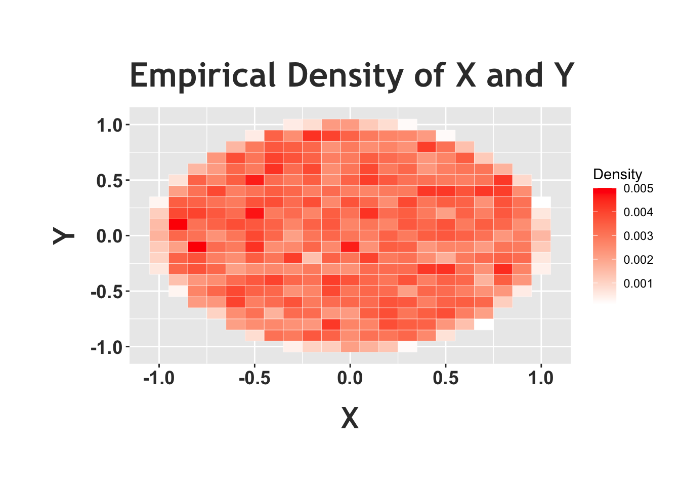
Notice how the above heat map, the empirical density, shows a circle with (relatively) the same color in the entire circle (of course, there appears to be some ‘noise,’ and small areas that are colored in differently, but that’s because this is a random simulation). This matches the ‘story’ we were trying to achieve; we want to randomly pick a point in the unit circle, and ‘random’ means that there should be the same density in every part of the circle, which means that the color of the heat map should be the same in all parts of the circle. To really see this in effect, we can plot the ‘analytical’ joint density with a heat map below. Recall that the joint PDF is just 1, so we should see the same color in the entire circle.
#define the supports/all combinations, from -1 to 1
X.a = seq(from = -1, to = 1, length.out = 100)
Y.a = seq(from = -1, to = 1, length.out = 100)
data = expand.grid(X.a = X.a, Y.a = Y.a)

#calculate density, just the product of Poisson PMFs (use dpois for the Poisson PMF)
data$density = apply(data, 1, function(x)
    1)

#remove points outside of the circle
data = data[data$X.a^2 + data$Y.a^2 <= 1, ]


#generate a heatmap
ggplot(data = data, aes(X.a, Y.a)) +
  geom_tile(aes(fill = density), color = "white") +
  scale_fill_gradient(low = "white", high= "red", name = "Density") +
  ggtitle("Analytical Density of X and Y") +
  theme(plot.margin = unit(c(1.8,.5,1.75,1.55), "cm")) +
  theme(plot.title = element_text(family = "Trebuchet MS",
            color="#383838", face="bold", size=25, vjust = 2)) +
  theme(axis.title.x = element_text(family = "Trebuchet MS",
            color="#383838", face="bold", size=22, vjust = -1.5),
        axis.title.y = element_text(family = "Trebuchet MS",
            color="#383838", face="bold", size=22, vjust = 2)) +
  theme(axis.text.x = element_text(face="bold", color="#383838",
                           size=14),
          axis.text.y = element_text(face="bold", color="#383838",
                           size=14))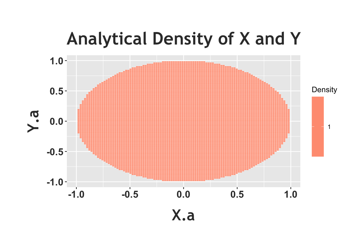
From here, we can try a common exercise related to joint distributions: marginalizing out one of the variables and thus recovering one of the marginal distributions. In this case, let’s find \(f(x)\) from \(f(x,y)\). This would be easy if the two were independent; however, does it appear that they are independent? It actually does not. Since we know that any two points \(x\) and \(y\) must satisfy \(x^2 + y^2 \leq 1\), knowing \(y\) could completely determine \(x\) (if \(y=1\), then \(x\) must be 0; if \(y\) is another point, then \(x\) can only be one of two points: if \(y = 0\), for example, then \(x=1\) or \(x=-1\)). Even if \(y\) and \(x\) were only related in this one case (in this example specifically, there are more cases) then the two random variables are not independent. So, instead, we’ll have to actually integrate \(y\) out. We’re integrating instead of summing because this is a continuous random variable and thus we have a PDF and not a PMF.
This is a pretty simple integral, but the one thing we have to be careful about is the bounds. That is, we’re not really letting \(y\) run from just -1 to 1: we’re bounding it such that it satisfies \(x^2 + y^2 \leq 1\) (if \(x = 1/2\), for instance, then letting \(y = 1\) would put us outside of the circle). Keeping that in mind, we’re going to get a function in the end with \(x\) in it, so we can’t just ignore \(x\) in the constraint. To contextualize, think about the double or triple integrals that you’ve done in the past in multivariable calculus: the inner variables have integrand bounds that include the outer variables. In this case, \(y\) has to have bounds that depend on \(x\). So, since \(x^2 + y^2 \leq 1\), we can solve for \(y\) and say that \(-\sqrt{1 - x^2} \leq y \leq \sqrt{1 - x^2}\). We integrate, remembering that the joint PDF is simply the constant \(\frac{1}{\pi}\):
\[f(x) = \int_{-\sqrt{1-x^2}}^{\sqrt{1-x^2}} \frac{1}{\pi} \; dy = \frac{y}{\pi} \Big|_{-\sqrt{1 - x^2}}^{\sqrt{1-x^2}} = \frac{2\sqrt{1 - x^2}}{\pi}\]
This is the marginal PDF of \(X\). It’s clear that the distribution of \(X\) is not uniform, since this PDF changes as \(x\) changes (it is a function of \(x\)) and we know that the Uniform PDF must be constant over the entire support/circle (i.e., does not change with \(x\)). Does it make sense that it’s not Uniform? It certainly does: there is simply more mass in the middle of the circle than at the edges. That is, if we pick a random point, it is more likely we’re somewhere in the middle than an extreme point on the side, so \(x\) values closer to 0 are more likely than \(x\) values closer to 1 or -1. You can think about it in terms of \(x\) and \(y\). Imagine if \(y = 0\): this means we have the interval \((-1, 1)\) on which to draw \(X\). This interval gets smaller and smaller the further we get from 0 (simply more mass in the middle); more on this below. Does this agree when we actually plug into the marginal PDF? Indeed it does. Clearly, plugging in 0 for \(x\) to the PDF will get a much larger value than if we plug in a number closer to -1 or 1, which would get us close to 0 (again, this is returning the density at a specific point).
In this case, if we wanted to recover the PDF of \(Y\), we wouldn’t have to go through and integrate \(x\) out; the two variables are essentially identical (i.e., a circle rotated 90 degrees is the same circle), so \(Y\) has the same PDF as \(X\), just with \(y\) replaced for \(x\). This is a powerful example of symmetry, which was introduced much earlier in the book but is still relevant amidst these more complex topics.
We can confirm this result (the marginal PDF of \(X\)) by checking if a simulation of \(X\) yields the same empirical density as the analytical density we just solved for. We will sample \(X\) and \(Y\) as we did before, and then compare densities.
#replicate
set.seed(110)
sims = 10000

#set paths for X and Y
X = rep(NA, sims)
Y = rep(NA, sims)

#run the loop
for(i in 1:sims){


  #go until we accept the sample
  while(TRUE){

    #sample x and y
    x = runif(1, -1, 1)
    y = runif(1, -1, 1)

    #see if we accept the sample
    if(x^2 + y^2 <= 1){

      #accept
      X[i] = x
      Y[i] = y

      #break, go to the next iteration
      break
    }
  }
}

#calculate analytical density
x = seq(from = -1, to = 1, length.out = 20)
dens = 2*sqrt(1 - x^2)/pi

#compare densities, should match
plot(density(X), main = "Density of X", col = "black",
     lwd = 3, xlab = "x", ylim = c(0, 1))
lines(x, dens, col = "red", lwd = 3, type = "p", pch = 16)

#make a legend
legend("topright", legend = c("Empirical PDF", "Analytical PDF"),
       lty=c(1,1), lwd=c(2.5,2.5),
       col=c("black", "red"))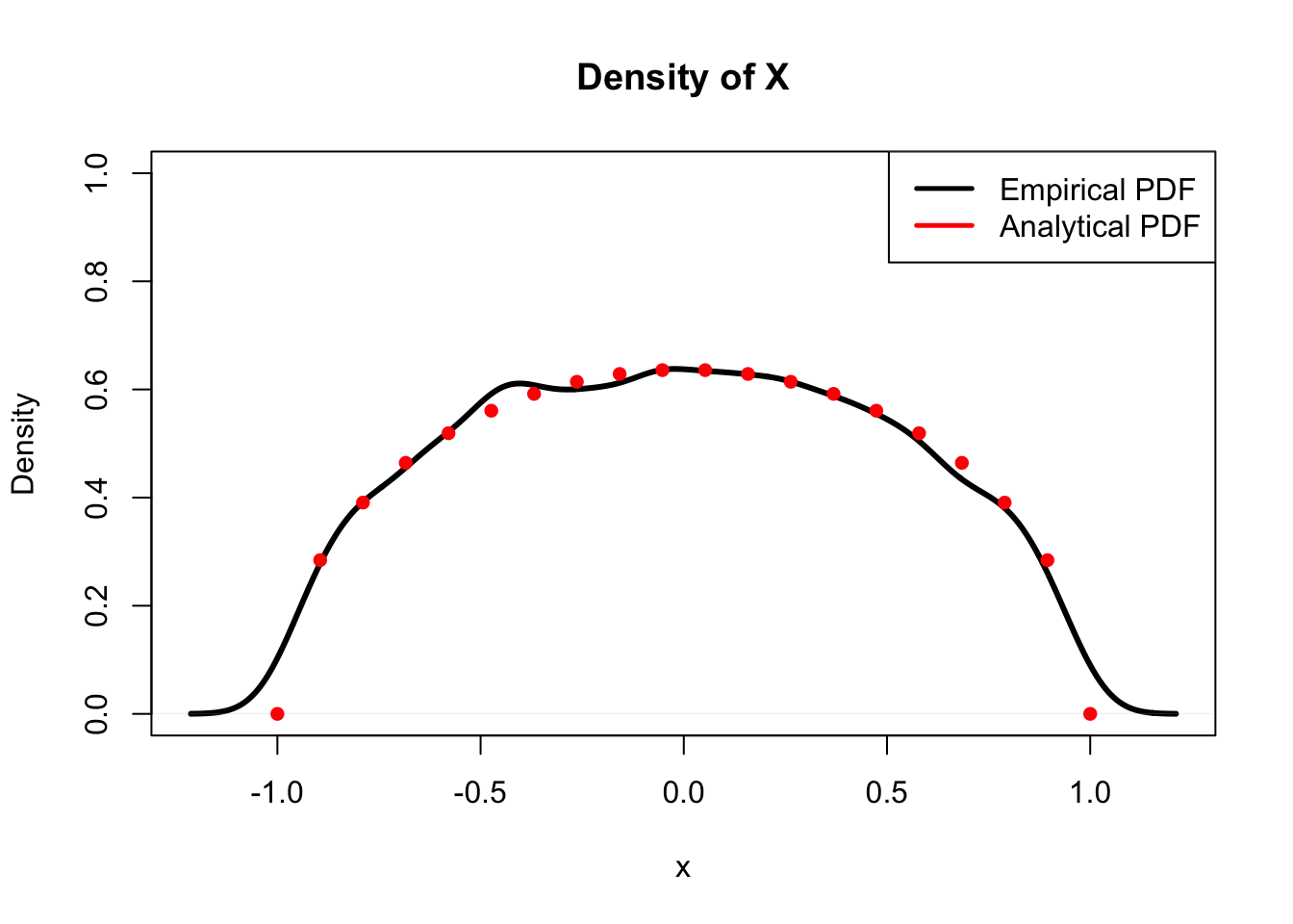
Hopefully by now the gist of joint distributions is clear. In the end, integrals and derivatives help us to navigate the multivariate landscapes of joint distributions. One major trap of joint PDFs is that it’s easy to assume random variables are independent, and thus the joint is the product of the marginals; this seems simple enough, but it’s so easy to forget that it’s worth mentioning again. Be sure to always be wary of independence of random variables, just as we are wary of assuming independence for simple probabilities! Another common hazard is working with the bounds when integrating from the joint to the marginal. Remember, just like standard double and triple integrals, the inner functions have bounds that include the outer functions (again, in this example, we had the bounds for \(y\) as a function of \(x\)).
We now move from joint to conditional distributions. Recall that a conditional probability is the probability that an event occurs given that another event occurred. Conditional distributions have the same property: it is the distribution of a random variable given that another random variable has crystallized to a specific value. This is written the same way as a probability: \(f(y|x)\), for example, gives the PDF of the random variable \(Y\) given the random variable \(X\), when \(X\) and \(Y\) are continuous. Can we write this in a different way? Recall the main rule of conditional probability:
\[P(A|B) = \frac{P(A \cap B)}{P(B)}\]
And, fortunately, we can adapt the same structure to random variables:
\[f(y|x) = \frac{f(x,y)}{f(x)}\]
That is, the conditional PDF of \(Y\) given \(X\) is the joint PDF of \(X\) and \(Y\) divided by the marginal PDF of \(X\).
It’s now clear why we discuss conditional distributions after discussing joint distributions: we need joint distributions to calculate the conditional distribution (the joint PDF is in the numerator!). This might seem a little vague, so let’s extend the example we used to discuss joint probability above. Given the same set up (remember, picking a random point from a circle) find \(f(y|x)\).
Fortunately, we’ve already done enough work to simply write down the answer almost immediately. That is, we know that the conditional PDF is just the Joint PDF of the two random variables divided by the marginal PDF of \(x\). We are thankfully given the Joint PDF from the start of the problem (\(\frac{1}{\pi}\)) and we solved for the marginal PDF of \(x\) above. Putting it together:
\[f(y|x) = \frac{\frac{1}{\pi}}{\frac{2}{\pi}\sqrt{1-x^2}} = \frac{1}{2\sqrt{1-x^2}}\]
This is the conditional PDF of \(Y\) given \(X\) for all \(y\) such that \(-\sqrt{1 - x^2} \leq y \leq \sqrt{1 - x^2}\) (i.e., the point is in the circle).
We can reflect on this conditional PDF to help build some intuition. An interesting thing to note is that this PDF does not depend on \(y\), just \(x\). Since \(x\) here is a given constant (conditioning on \(X\) means that we know that it crystallized to some value \(x\)), and this is a PDF of \(y\), this means that \(Y\) conditioned on \(X\) is Uniform! That is, for a given value of \(x\) (and of course, values of \(x\) are given, since this is the distribution of \(Y\) conditioned on the random variable \(X\)), the PDF is completely constant in that it does not change with \(y\) (not a function of \(y\)). Does that make sense? This is actually an intuitive result: after all, we are looking for the distribution of \(Y\) given some fixed value of \(x\). Envision picking a value of \(x\) for \(X\) to crystallize to. Then, conditioned on this value, \(Y\) is generated randomly somewhere on that vertical line. For example, say that we fix \(X\) such that \(x=0\). Given this, we know that \(Y\) can take on a value on the vertical line \(x=0\) from the point (0,-1) to the point (0,1), or anywhere between \(-1\) and \(1\). We already know that \(Y\) is not uniform marginally; it’s more likely to take on a value somewhere near the middle of the circle simply because there is more mass there. However, it makes sense that \(Y\) is uniform conditioned on \(X\), since once we fix the value of \(x\), we know that \(Y\) is just generated randomly on that vertical line where the upper and lower bounds are just the bounds of the circle. As discussed above, the length of the interval that we generate \(Y\) on (the support of this conditional distribution) shrinks as \(x\) gets to the endpoints.
Hopefully this not only helped in figuring out how to find the conditional distribution but for thinking about how it actually works. Again, while the joint distribution is just picking a point randomly in a circle and then taking those \(x\) and \(y\) coordinates, the conditional actually fixes an \(x\) value first and then randomly generates a \(y\) value. You may find it helpful to draw this out on an actual graph if you are still struggling with the visual.
In fact, we can check our result using a similar simulation in R: we’ll generate values for \(X\) and \(Y\), then plot the density of \(X\) conditioned on some value of \(Y\) (technically, we’ll condition on \(Y\) being in some small interval, since the probability that it takes on any value exactly is 0 because it is a continuous random variable). We should see that the density is uniform.
#replicate
set.seed(110)
sims = 10000

#set paths for X and Y
X = rep(NA, sims)
Y = rep(NA, sims)

#run the loop
for(i in 1:sims){


  #go until we accept the sample
  while(TRUE){

    #sample x and y
    x = runif(1, -1, 1)
    y = runif(1, -1, 1)

    #see if we accept the sample
    if(x^2 + y^2 <= 1){

      #accept
      X[i] = x
      Y[i] = y

      #break, go to the next iteration
      break
    }
  }
}


#condition on a specific value of x
cond.x = 0

#define a title
title = paste0("Density of Y|X is near ", cond.x)

#calculate analytical density
y = seq(from = -1, to = 1, length.out = 10)
dens = rep(1/(2*sqrt(1 - cond.x^2)), length(y))

#the conditional density (conditioned on y in a small interval) should be uniform
# and should match our analytical result
plot(density(Y[X < cond.x + 1/10 & X > cond.x - 1/10]),
     main = title, col = "black", ylim = c(0, .8),
     lwd = 3, xlab = "y")
lines(y, dens, col = "red", lwd = 3, type = "p", pch = 16)

#make a legend
legend("topright", legend = c("Empirical PDF", "Analytical PDF"),
       lty=c(1,1), lwd=c(2.5,2.5),
       col=c("black", "red"))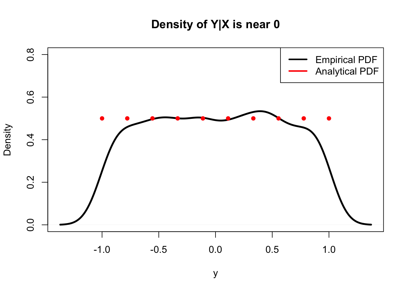
Hopefully this provided an enlightening discussion of joint and conditional distributions. Refer back to all of the properties of a joint distribution to build more intuition, and remember that the conditional distribution can be found with the joint and the marginal (similarly to how we use joint and marginal probabilities to find conditional probabilities).
2-D LoTUS
Now that we are masters of joint distributions - multivariate extensions of marginal distributions - we need an extension of LoTUS as well. Specifically, we need ‘2-D LoTUS.’ The LoTUS we used before was officially called 1-D LoTUS (although we never explicitly referred to it as such) because it dealt with only one variable/distribution. This 2-D version, clearly, deals with 2 variables (and you can keep generalizing as you add variables so that 2-D LoTUS becomes \(n\)-D LoTUS, if necessary).
Like its one-dimensional partner, 2-D LoTUS is used in finding expectations of random variables (and, eventually, expectations of functions of random variables). The expectation is found in a very similar way: recall how, using LoTUS, we just multiplied the function that we were trying to find the expectation of by the PDF and integrated? In the two dimensional case, we simply multiply the function of both variables by the joint PDF and integrate over the supports of both variables. Officially, if we have two random variables \(X\) and \(Y\) with Joint PDF \(f(x,y)\), and we have some function \(g(x,y)\) (one example would be something like \(2xy^4\)) then we could find the expectation of the function with LoTUS:
\[E(g(X,Y)) = \int_{-\infty}^{\infty} \int_{-\infty}^{\infty} g(x,y) f(x,y) \; dx \; dy \]
Here, we integrate from negative infinity to infinity to be as general as possible; of course, in an actual example, we would only integrate over the support, which might be less extreme than the infinities in the bounds here (however, it never hurts to integrate over all real numbers, since if the PDF is defined correctly, any value that is not in the support has no density and will simply return a value of 0).
This is a relatively natural extension and hopefully not too big a jump; just to solidify the concept, though, let’s consider an example.
Example 6.1 (product of Uniforms):
Let \(U_1\) and \(U_2\) be i.i.d. Standard Uniform random variables. What is \(E(U_1 \cdot U_2)\)?
Before we start, do you have any intuition on what this should be? We know marginally that both r.v.’s have an expectation of .5, so you might guess that the product of the r.v.’s has expectation \(.5^2 = .25\). This is by no means a rigorous way to answer the problem, just a way to build intuition to see if our solution matches when we actually perform the calculation.
Anyways, this turns out to be a pretty straightforward example, but let’s think about what we need. First, we need the joint PDF; thankfully, the two random variables are independent (we are given that they are i.i.d.), so we can just multiply the marginal PDFs. Further, the marginal PDF of a Standard Uniform is simply 1 (recall that \(f(u) = \frac{1}{b-a}\), and \(a\) and \(b\) are 0 and 1 in this case). So, the product of the marginal PDFs, or the joint PDF, is just 1.
We then need to multiply this simple Joint PDF by the function of the two variables and integrate over the bounds. In this case, the function is simply multiplying the two random variables (since we are finding the expectation of \(U_1 \cdot U_2\)), and the bounds are simply 0 to 1 for each random variable (we do not have to write the bound of the inner integral in terms of the variable in the outer integral, since these random variables are independent and thus their bounds are unrelated). We write:
\[E(U_1 U_2) = \int_{0}^{1}\int_{0}^{1} u_1 u_2 \; \; du_1 du_2\]
This is an easy double integral. Working through it, we get:
\[\int_{0}^{1}\int_{0}^{1} u_1 u_2 \; \; du_1 du_2 = \frac{1}{2} \int_{0}^{1} u_2 \; \; du_2 = \frac{1}{4}\]
So, the expected value of the multiplication of two Standard Uniforms is just \(1/4\). This matches our intuition, because, like we said above, we know that the expected value of a Standard Uniform random variable is one half, and multiplying two expectations would yield \(\frac{1}{4}\). Many times, our intuition is not be matched by the eventual result, so enjoy this intuitive result that is also actually correct!
We can check our result very quickly in R, by generating values from two independent standard uniforms and finding the mean of their product.
#replicate
set.seed(110)
sims = 1000

#generate the r.v.'s
U1 = runif(sims)
U2 = runif(sims)

#combine into a product (call it X)
X = U1*U2

#should get 1/4
mean(X)
## [1] 0.2396835We saw that we arrived at the intuitive answer (the mean of the products was the product of the means), but be sure not to over-extend this result. The above seems like a fast way to the Expectation of the product of random variables: just multiply the Expectation of both random variables. However, while the intuition was enticing in this case, intuition is not an actual proof. Instead, let’s actually prove it using 2-D LoTUS. This will not only solidify your understanding but will get us a pretty valuable result that we can use in the future.
Let \(X\) and \(Y\) be independent random variables, and imagine that we want to find \(E(XY)\); similar to the case above with the two Uniforms, but more general (\(X\) and \(Y\) can have any distributions). We can indeed use 2-D LoTUS here, since \(E(XY)\) is basically a function of the two variables \(x\) and \(y\): it’s simply \(x \cdot y\). So, if \(X\) and \(Y\) have a joint PDF given by \(f(x,y)\), we can find the expectation by writing:
\[E(XY) = \int_{-\infty}^{\infty} \int_{-\infty}^{\infty} xy f(x,y) \; dx \; dy \]
However, we are given that \(X\) and \(Y\) are independent, which means the Joint PDF is simply the product of the two marginal PDFs; that is, \(f(x,y) = f(x)f(y)\). We can thus re-write:
\[E(XY) = \int_{-\infty}^{\infty} \int_{-\infty}^{\infty} xy f(x)f(y) \; dx \; dy \] And since we are integrating with respect to \(x\) first, the \(y\) and \(f(y)\) are constant terms (they don’t change with \(x\)) and can be brought out behind the first integrand:
\[E(XY) = \int_{-\infty}^{\infty} xf(x) \; dx \int_{-\infty}^{\infty} y f(y) \; \; dy \]
Now, we have arrived at a point that looks like the product of the expectation of \(X\) and the expectation of \(Y\), from 1-D LoTUS. So, we can finally write:
\[E(XY) = E(X)E(Y)\]
If \(X\) and \(Y\) are independent.
This is exactly what we saw with the Uniforms and kind of a similar result to what we’ve seen so far; if independent, just multiply! We’ve seen this result with probabilities and density functions, and now we see it with expectation. Officially, this is a very important result that states if \(X\) and \(Y\) are independent random variables, then \(E(XY) = E(X)E(Y)\), or the expectation of the product is just the product of the expectations. We’ll delve into the concept of ‘covariance’ later, but this example essentially says that independence implies two random variables have a covariance of 0 and thus are un-correlated (we will explore this more in Chapter 7).
Remember, though, that we can’t extend this result to dependent random variables. Imagine \(I_H\) and \(I_T\), which are indicator random variables that the flip of a random coin is heads and tails, respectively. If we applied the above formula to finding \(E(I_H I_T)\), we would get \(E(I_H)E(I_T) = 1/4\). However, by looking at this product, we can realize that every time \(I_H\) is 1, \(I_T\) is 0 (if we get a heads, we don’t get a tails), and vice versa, so \(I_H I_T\) is always 0 and \(E(I_H I_T) = 0\). Clearly, the dependent case requires a bit more work than just multiplying expectations! In the proof presented above, the dependent case ‘breaks’ the calculation because \(f(x, y)\) does not simply factor to \(f(x) \cdot f(y)\) (a step that allows us to consider the integrals separately).
Anyways, the main point of this exercise was to get familiar with 2-D LoTUS; it’s really the same as the LoTUS that we’ve been using all along: just multiply the function by the Joint PDF and integrate! If \(A\) was Poisson distributed and \(B\) was independently Exponentially distributed, how do you find \(E(\frac{a}{b})\)? Simply take \(\frac{a}{b}\) times the product of a Poisson PMF times an Exponential PDF, integrated over the supports! How would you find the expected squared difference between two Standard Uniforms? Integrate the squared absolute value of the difference of the two random variables times the joint PDF, which is just 1, over the bounds \(0\) and \(1\). Clearly, this tool can apply to many different types of problems.
Multinomial
The Multinomial is a great distribution because it’s not too challenging conceptually; it really just expands upon what we’ve learned so far. In fact, it fits in very well with the major underlying theme of this chapter: so far we have looked at concepts developed earlier on, generalized to higher dimensions (multiple marginal distributions become joint distributions, one dimensional LoTUS becomes two dimensional, etc.). We’ll continue along the same lines here.
The Multinomial is a higher dimensional Binomial. Of course, by this point, we are familiar with the Binomial and are quite comfortable with this distribution. The Story of the Multinomial goes that if you have \(n\) independent trials, and each trial has \(k\) outcomes, each with a fixed probability \(p_k\) of occurring, then the outcomes (which we generally write into one vector) follow a Multinomial distribution. You can probably see where the generalization comes in: with the Binomial, we only had two outcomes, success or failure. For the Multinomial, there’s no limit to the number of outcomes. Imagine, instead of flipping a coin for the Binomial where there are only two outcomes (heads or tails), rolling a die with 6 possible outcomes for the Multinomial (also, instead of “Bi” as the prefix, which generally means 2 outcomes, we have “Multi”; pretty intuitive, no?). You could also imagine taking \(n\) objects and putting them one at a time randomly in one of \(k\) boxes, where there are constant probabilities of putting an object into each box (all of these probabilities must sum to 1, since you must put each object in a box!). Of course, the Binomial ‘version’ here would just be taking \(n\) objects and placing them in 2 boxes (each with fixed probabilities that sum to 1, etc.). This is a helpful paradigm for the Multinomial because each object can only be placed in 1 box, which is a key part of the distribution. It’s actually pretty similar to how the Negative Binomial is an extension of the Geometric. The Geometric waits for just 1 success, while the Negative Binomial generalizes to multiple successes. Here, the Multinomial generalizes the Binomial to more than 2 outcomes on each trial, instead of just the usual ‘success or failure.’
Formally, the Multinomial is a multivariate discrete distribution (we’ll see multivariate continuous distributions later when we discuss the multivariate normal); essentially a joint distribution for multiple random variables. Specifically, you might have \(\vec{X} \sim Mult(n,\vec{p})\) where \(\vec{X}\) is the vector of random variables \(\{X_1,X_2, ... X_k\}\) and \(\vec{p}\) is the vector of probabilities \(\{p_1,p_2,...p_k\}\) that each outcome occurs. You can think of this as if there are \(k\) different outcomes, represented by the random \(X\) vector, and each outcome has a certain probability/each random variable has a different parameter, represented by the terms in the \(p\) vector So, \(P(X_1)\), which we can think of as the probability of the first outcome occurring (i.e., a ball is placed in the first box), is \(p_1\) (think about rolling a fair die; there are six events, rolling 1 through 6, and the first event, rolling a 1, has probability \(p_1 = \frac{1}{6}\)). We know for all \(j\) that \(0 \leq p_j \leq 1\), since these are valid probabilities, and, as mentioned above, that \(\sum_{j} p_j = 1\), since they must cover all possible outcomes (if the sum of all \(p\)’s was .9, we wouldn’t know what the outcome was \(10\%\) of the time!).
This might seem a little complicated, but think of rolling a fair die 10 times, and call that random variable \(\vec{R}\), where \(\vec{R}\) is a vector that counts the number of outcomes for each roll (i.e., the first entry in the vector is the number of times that we rolled a 1, the second entry is the number of times that we rolled a 2, etc.). If we are interested in counting the number of each of the six rolls (count the number of 1’s rolled, the number of 2’s rolled, etc.), we can say that \(\vec{R} \sim Mult(10,\vec{p})\), where of course \(\vec{p}\) is the probability vector that gives probabilities of success for all the outcomes of the die. Since it is a fair die, all six outcomes are equally likely and thus \(\vec{p} = \{\frac{1}{6}, \frac{1}{6},\frac{1}{6},\frac{1}{6},\frac{1}{6},\frac{1}{6}\}\).
If all of this notation is jarring you, just think again that we are essentially working with a Binomial, but instead of just success or failure we have more than 2 different outcomes. Let’s focus now on the PMF of the Multinomial. Essentially, it is a joint PMF made up of multiple random variables, since we are finding the probability that all of the \(X\) random variables take on certain values. That is, in our notation:
\[P(X_1 = n_1 \cap X_2 = n_2 \cap ... \cap X_k = n_k)\]
Although, as we mentioned earlier, commas are usually used instead of \(\cap\).
Can you envision why this makes sense? Well, if we go back to our die roll example of a Multinomial, you could say that there are six different random variables, \(X_1\) through \(X_6\), where each one represents the number of times that the respective number is rolled on the die. So, a specific outcome of this Multinomial random variable might be rolling three 1’s, four 2’s and no other numbers. In that example, we would write the probability as:
\[P(X_1 = 4, X_2 = 4, X_3 = X_4 = X_5 = X_6 = 0)\]
You can see why the ‘joint’ PMF makes sense; we are taking the probability that many different random variables take on specific values.
So, what is this Joint PMF? In the most general case, we can write it as:
\[P(X_1 = n_1 \cap X_2 = n_2 \cap ... \cap X_k = n_k) = \big(p_1^{n_1} p_2^{n_2}...p_k^{n_l}\big) \Big(\frac{n!}{n_1!n_2! ... n_j!} \Big)\]
Does this make sense? You will find that this is in fact a simple application of the probability and counting techniques you are already very familiar with. Let’s consider the first part, the probabilities multiplied together: \(\big(p_1^{n_1} p_2^{n_2}...p_k^{n_l}\big)\) . This makes sense, since we know that the probability that event 1 occurs \(n_1\) times is just \(p_1\) multiplied by itself \(n_1\) times, and the same for event 2, 3, all the way up to \(k\). We also know that since all of the trials are independent, we can multiply the probabilities, and thus we get this expression. This is the same as the \(p^k (1 - p)^{n-k}\) term in the Binomial PMF, except, of course, generalized to many \(p\)’s instead of just \(p\) and \(1 - p\).
However, this term only gives the probability of one possible permutation (i.e., there are multiple ways to roll four 2’s and two 1’s in six rolls of the die: 222211 and 112222 are different but are both valid) so we must count all of the possible permutations and multiply by the probability of each permutation (they all have the same probability; think about how 222211 and 112222 have the same probability of occurring). Well, consider the number of ways to order 222211. As we’ve learned, if the numbers were all distinct, there are 6! ways to order them. However, we are overcounting, since all of the 2’s are the same and all of the 4’s are the same. How do we correct this? Since the 2’s are interchangeable among themselves and the 4’s are interchangeable among themselves, we just divide out those factorials: \(\frac{6!}{4!2!}\) (i.e., you could rewrite 222211 by rearranging the 2’s, but it would be the same thing: 222211. We don’t want to count this rearranging as a legitimately different iteration). This is the exact same problem as counting the ways to order the letters in STATISTICS; the factorial for the number of total letters divided by the factorials for the repeat letters. This gives us the second term, \(\Big(\frac{n!}{n_1!n_2! ... n_l!} \Big)\), and all of the sudden the PMF makes sense.
It’s also possible to work with the Multinomial in R; this can help to solidify our understanding of the distribution. We can use rmultinom to generate random values (like rbinom) and dmultinom to work with the density (like dbinom). We just have to be sure to enter the number of boxes (possible outcomes) we want, the number of trials we want to have for each experiment and the number of experiments we want to run. Here, we define the probability vector \(c(.05, .3, .5, .15)\) and use it as the third argument in rmultinom. The length of this vector indicates how many outcomes we want our Multinomial random variable to have; here, we have a vector of length 4, meaning the Multinomial has 4 possible outcomes (the first possible outcome has probability .05, etc.). From here, we define \(x = 3\) and use this as the second argument; this tells us how many trials we have. So, in this case, we have 4 ‘boxes’ (length of the probability vector is 4) and we want to put \(x = 3\) balls in these boxes (based on the given probability vector). Finally, we define \(n = 10\), meaning we want to run the entire experiment 10 times (i.e., putting all 3 balls into the 4 boxes counts as 1 experiment, and we want to do this 10 times). You can see how the output matches the arguments we entered: we have a 4x10 matrix, where every column represents a single experiment. Consider the first column. This is saying that on the first run of the experiment, we put 2 balls in box 3 (i.e., had ‘outcome 3’ twice) and 1 ball in box 4 (i.e., had ‘outcome 4’ once). The columns will always sum to 3, since it is counting the number of balls we put in the boxes.
#replicate
set.seed(110)

#define parameters; n is number of draws, k is number of outcomes
n = 10
x = 3

#define probability vector
prob.vector = c(.05, .3, .5, .15)

#generate random values
rmultinom(n, x, prob.vector)
## [,1] [,2] [,3] [,4] [,5] [,6] [,7] [,8] [,9] [,10]
## [1,] 0 0 1 0 0 1 0 1 0 0
## [2,] 0 1 2 1 1 0 1 1 3 0
## [3,] 1 2 0 1 1 2 2 0 0 2
## [4,] 2 0 0 1 1 0 0 1 0 1So, these are the general characteristics of the Multinomial, but, given that it is a multivariate distribution (remember, this just means a joint distribution of multiple random variables) there are interesting extensions that we can tack on. For example, we saw that a Multinomial is made up of a vector of dependent, jointly distributed \(X_j\)’s. You can think of each \(X\) as a specific outcome, and each has a certain probability of success and failure (\(p_j\) is the probability of success). So, a pretty interesting result is the marginal distribution of \(X_j\) for a \(Mult(n,\vec{p})\) random variable:
\[X_j \sim Bin(n,p_j)\]
Given this, we know \(E(X_j) = n p_j\), and \(Var(X_j) = np_jq_j\).
That makes a lot of intuitive sense, and there are a of couple ways to think about this result. Consider first the tried and true example of rolling the fair die 6 times. You could model this as a Multinomial random variable: we have repeated, independent trials with outcomes 1 through 6. However, if you consider one outcome marginally, like the outcome of the die rolling a 1, it makes sense that this random variable is Binomial. It has a specific probability of success or failure and a set number of independent trials (here, 10 trials). So, the Multinomial is just the joint distribution of different Binomial distributions (remember, though, we still have the constraint that all of the probabilities in the Multinomial must sum to 1). Importantly, these Binomial random variables are dependent. Consider (in the context of the example above) the random variable that tracks how many rolls of the die are 1 vs. the random variable that tracks how many rolls of the die are 6. Both are marginally Binomial as we saw. If we observe that the first random variable takes on the value 10 (i.e., we roll ten 1’s) then we know that the second random variable takes on the value 0 (since all of the rolls are 1, so none can be 6). This means that the random variables must be dependent.
Let’s push a little farther and introduce another important Multinomial concept: Lumping. This is pretty much exactly what it sounds like: we lump together multiple outcomes to create one large outcome. For example, in the classic fair die roll, lumping together the outcomes of rolling a 4, 5 or 6 would essentially be lumping them into the one event of “rolling greater than a 3.” This does not affect the distribution; we are still working with a Multinomial random variable. That makes good sense, because we still have a vector of outcomes, each with an associated probability; we’ve just combined some outcomes into one, but we can still put this ‘new’ outcome into our vector of outcomes. In fact, we know the probability of this large, lumped outcome: it’s just the sum of the probabilities of the outcomes that went ‘into’ the lump! That is, the probability of the lumped outcome “rolling a three or greater” on a fair die is the sum of the probabilities of each outcome on the die that is greater than three: the probability of a 4 plus the probability of a 5 plus the probability of a 6. Of course, this comes out to \(\frac{1}{6} + \frac{1}{6} + \frac{1}{6} = \frac{1}{2}\). Officially, if \(C = B + A\), then \(P(C) = P(B) + P(A)\) (this holds if \(A\) and \(B\) are disjoint; we know that this condition is satisfied for the Multinomial because only one outcome can occur at a time, or each of the \(k\) objects can only go into one box, as stated earlier. You can’t roll a 4 and a 2 in one roll of the dice!).
Let’s formalize this concept with some notation. If we start with a Multinomial random variable with outcomes 1 through \(k\) and probabilities \(p_1\) through \(p_k\) and you want to lump, say, the third outcome onwards, all the way to the final \(k^{th}\) outcome, the ‘lumped’ random variable is still a Multinomial. The original random variable would look like:
\[\vec{X} = \{X_1,X_2, ... , X_k\} \sim Mult(n,\{p_1,p_2,...,p_k\})\]
Then, if we lump the third through the \(k^{th}\) outcomes together and call this new random variable \(\vec{Y}\), we can write:
\[\vec{Y} = \{X_1,X_2, X_3 + X_4 + ... + X_k\} \sim Mult(n, \{p_1,p_2, p_3 + p_4 + ... + p_k\})\]
That is, now we have three outcomes: \(X_1\), \(X_2\), and the rest of the outcomes (3 through \(k\)) lumped into one. The probabilities change, since the probability of this big lumped outcome is just the sum of the probabilities of the individual outcomes making up the large lumped outcome. However, the probabilities still add to 1.
As a quick check, this ‘lumped’ Multinomial is made up of three Binomials: \(X_1 \sim Bin(n,p_1)\), \(X_2 \sim Bin(n,p_2)\), and \(X_3 + X_4 + ... + X_k \sim Bin(n,p_3 + p_4 + ... + p_k)\). Convince yourself that this is correct, based on the work we did before the ‘lumping’ section.
Finally, let’s think of the Multinomial conditionally. That is, if \(\vec{X} \sim Mult(n,\vec{p}\)), what is the conditional distribution of \(\vec{X}\) given that \(X_1 = n_1\)? We can think of this as the distribution of the remaining die rolls in 10 total rolls of a fair die given that a 1 is rolled three times.
This just takes a little bit of thinking to figure out. To start, we have a different number of trials now; in total, we are now working with \(n - n_1\) trials. That is, given that \(X_1\) occurred \(n_1\) times, we have \(n-n_1\) trials left over to work with (in the example above, given that we have rolled a 1 three times out of 10 rolls, we have 10 - 3 = 7 rolls left over. So, that’s the first parameter of our Multinomial: the number of trials, or \(n - n_1\)).
Now we need to find the probabilities of the remaining outcomes. It might seem that they are the same; just \(p_2\) through \(p_k\). However, recall the fundamental concept of conditional probability: parsing down the sample space and thus changing the structure of the problem. Since we are given that some event occurred, the overall sample space shrinks. In this case, we have taken out the first outcome, which eliminates \(p_1\), and thus the entire ‘probabilistic sample space’ is no longer 1 but \(1 - p_1\). That is, the probability that \(X_2\) occurs is no longer \(p_2\), but \(\frac{p_2}{1 - p_1}\). We have to normalize the probabilities (re-weight them so that they sum to 1) because there is no possibility of \(X_1\) occurring, and thus the rest of the outcomes become more probable (if \(X_1\) had a non-zero probability of occurring, that is!). So, officially, given that \(X_1 = n_1\), we can write:
\[\{X_2, X_3, ... X_k\} \sim Mult(n - n_1, \{\frac{p_2}{1 - p_1}, \frac{p_3}{1 - p_1},...,\frac{p_k}{1 - p_1} \})\]
As well as being an interesting result, this is a great way to show that the Binomials that make up the Multinomial are not independent, which we discussed intuitively above. Observing the outcome of one Binomial random variable gives information about the rest of Binomial random variables; the probability parameter of these random variables change. This make sense. Recall the example above: if we are rolling a fair, 6-sided die 10 times and we condition on rolling ten 1’s (the first Binomial) then we know that the other five Binomials (which count the number of rolls that crystallized to 2 through 6) all took on value 0.
We can confirm this intuition with a simulation in R. Imagine a Multinomial with 3 outcomes and equal probabilities of each outcome. We’ll condition on a specific number of outcomes in the first ‘bucket’ and, conditioned on this, examine the distribution of the number of outcomes in the second ‘bucket.’ Based on the above result, this distribution should be Binomial. In this example, we will consider a Multinomial with 3 ‘buckets’ and 5 ‘balls’ to put in the buckets. We call the buckets \(X\), \(Y\) and \(Z\) and consider the distribution of \(X\) conditioned on \(Y = 0\). Based on the above, we should have \(X \sim Bin(5, \frac{1/3}{1/3 + 1/3} = 1/2)\).
#replicate
set.seed(110)
sims = 1000

#draw the data
data = rmultinom(sims, 5, prob = c(1/3, 1/3, 1/3))

#call the rows X, Y and Z (different buckets)
X = data[1, ]
Y = data[2, ]
Z = data[3, ]

#histograms should match

#set 1x2 graphing grid
par(mfrow = c(1,2))

#plot X
hist(X[Y == 0], main = "X|Y = 0", col = rgb(1, 0, 0, 1/4), xlab = "", breaks = 0:5)
hist(rbinom(sims, 5, 1/2), main = "Bin(5, 1/2)", col = rgb(0, 1, 0, 1/4), xlab = "", breaks = 0:5)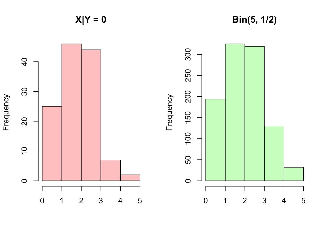
#restore graphing grid
par(mfrow = c(1,1))
This closes our discussion of the Multinomial. It’s important to remember the story of this distribution, and, as with discrete distributions we learned about early on, helpful to understand the PMF. It’s also very useful to remember some of its interesting properties: how the marginal distributions are Binomial, how you can lump outcomes together, and how the distribution changes conditionally. The last thing to touch on is how the Binomial is a degenerate case of the Multinomial, just like \(Bern(p)\) is the same as \(Binom(1,p)\) (making the Bernoulli a very degenerate Multinomial) and \(Geom(p)\) is the same as \(NBinom(1,p)\). Convince yourself that if you just had two ‘boxes’ in the Multinomial (your vector of boxes and your vector of probabilities both had length 2) then the PMF reduces and becomes the same as the Binomial PMF. This makes sense; we’re drawing random outcomes and putting them in one of two boxes, which we could even label as success or failure.
Chicken and Egg
Which came first? It’s an age old question, and the true answer (or, maybe just the most interesting answer) is that a circle has no beginning. Anyways, this is simply the name of a really interesting characteristic of the Poisson distribution.
Let’s set up the problem that drives this property. Say that a chicken lays \(N\) eggs, where \(N\) is a random variable that follows a Poisson distribution such that \(N \sim Pois(\lambda)\). It’s key that \(N\), the total number of eggs, is a random variable (i.e., we don’t have a fixed number of eggs). Each egg hatches independently with probability \(p\). Let \(X\) be the number of eggs that hatch, and \(Y\) be the number of eggs that don’t hatch. Find the Joint PMF of \(X\) and \(Y\). We’ll solve this with a similar approach that Professor Blitzstein uses in this freely available lecture.
Right off of the bat, we can envision what exactly the ‘Joint PMF’ represents. We know we can write it as \(P(X=x,Y=y)\), since \(X\) and \(Y\) are discrete, and we can think of it as the probability that a certain number of eggs hatch and a certain number don’t. At first glance, it seems that these two are not independent; the more eggs that hatch, you would think, the less that are likely to not hatch (remember, we don’t know how many eggs there are in total, because \(N\) is a random variable). However, this intuition is not a proof, and we’ll have to actually check this result. If we knew how many eggs the chicken laid, then knowing the number of eggs that hatched would of course give us the number that didn’t hatch (that is, knowing \(X\) and \(N\) determines \(Y\)). But, again, the key is that \(N\), the number of laid eggs, is itself random.
Before we start, there are a couple of useful pieces of info that we can glean from the problem statement above. Since eggs can either hatch or not hatch (there are no other options), we know that \(X + Y = N\) (remember, again, these are all random variables). Given some value for \(N\) (that is, if we somehow know the number of eggs that there are), we could say that \(X\) and \(Y\) are Binomial random variables, since we have a set number of trials (\(N\) eggs) and each has the same probability of hatching or not, \(p\). So, we could write \(X|N \sim Bin(N,p)\), and \(Y|N \sim Bin(N,1-p)\), by the story of the Binomial distribution.
Now, though, we’re a bit stuck. This is a perfect opportunity for us to use conditioning, or exercise ‘wishful thinking’: is there something that we wish we knew? If we can identify something that we ‘wish we knew,’ then we can condition on it. The obvious choice here is to condition on \(N\), the total number of eggs, since if we are given this value then we know the distributions of \(X\) and \(Y\). Recalling our work with the LOTP, which in its simplest form states that \(P(A) = P(A|B)P(B) + P(A|B^c)P(B^c)\), we can write, for specific \(i\) and \(j\):
\[P(X = i, Y = j) = \sum_n P(X=i,Y=j|N=n)P(N=n)\]
Remember that we have to get rid of the unwanted variable, or \(N\), by summing it out of this expression (akin to what we would do with LOTP. We’ve generally worked with only two ‘partitions’; the above is just extending to more partitions).
Anyways, this makes sense, since all we are doing is taking the joint distribution of \(X\) and \(Y\) and conditioning on the value that \(N\) takes on (notated by \(n\), as usual). Then, by the LOTP, we weight the expression by the probabilities that \(N\) actually takes on \(n\). This marginalizes out the random variable \(N\), and we are left with the joint PMF of \(X\) and \(Y\).
Where do we go from here? Well, recall that we already know at least one identity between \(X\), \(Y\) and \(N\). Eggs can either hatch or not hatch, so \(X + Y = N\). That means that for any values \(i\) and \(j\) that \(X\) and \(Y\) take on, \(N\) must be the sum of \(i\) and \(j\) (after all, if 5 eggs hatched and 2 didn’t hatch, then there must have been 7 eggs to start with). So, we could rewrite our problem without the full summation:
\[P(X = i, Y = j) = P(X=i,Y=j|N= i + j)P(N=i + j)\]
All we did was simplify the sum down to one expression, because the probability is 0 everywhere else (for example, if \(N = 10\), the probability is 0 that \(X = 1\) and \(Y = 2\)). This still doesn’t look like a simple calculation, but we can again make good use of the identity \(X + Y = N\). That is, if \(N = i + j\), and \(X=i\), then \(Y\) must be equal to \(j\). So, writing \(Y = j\) in the \(P(X=i,Y=j|N= i + j)\) is just redundant. We can simply write:
\[= P(X=i|N= i + j)P(N=i + j)\]
And we are almost there, because we know these two distributions. First, we know that \(X\) given \(N\) is just a Binomial random variable, so the distribution of \(X\) given \(N = i + j\) is just \(Bin(i+j,p)\). We also know the distribution of \(N\) is \(Pois(\lambda)\), from the prompt. Given this, we can simply write out the PMFs of the two distributions and multiply them (remember, we are writing out \(P(X = i|N = i + j)\) and \(P(N = i + j)\), knowing that \(X\) is Binomial given \(N\), and that \(N\) is marginally Poisson):
\[\Big({i + j \choose i} p^i q ^ j\Big) \; \Big( \frac{e^{-\lambda}\lambda^{i+j}}{(i+j)!}\Big)\]
The term on the left is the PMF of the Binomial random variable and the term on the right is the PMF of the Poisson random variable.
Now that we actually have a closed form representation, all we have to do is simplify (it’s good practice to work through this algebra yourself, and it’s relatively straightforward: try plugging in the definition of \({i + j \choose i}\), or \(\frac{(i + j)!}{i!j!}\) first). Here, we’re just going to write what this simplifies out to:
\[P(X = i, Y = j) = \Big(e^{\lambda p} \frac{(\lambda p)^i}{i!}\Big) \Big(e^{\lambda q}\frac{(\lambda q)^j}{j!} \Big)\]
Voila! This might not seem so spectacular at first, but realize that this is actually the product of the PMF of two Poisson random variables. Specifically, two Poisson random variables with parameters \(\lambda p\) (on the left) and \(\lambda q\) (on the right), respectively. What does that mean? Well, it means the distribution of \(X\) is \(Pois(\lambda p)\), and the distribution of \(Y\) is \(Pois(\lambda q)\) (remember, \(\lambda\) is the original parameter of the Poisson \(N\)). And, since the joint PMF (remember, that’s what we were trying to find this whole time) just simplifies down to the product of these two PDFs (which we can tell because we can factor out the \(i\) terms that are associated with \(X\) and the \(j\) terms that are associated with \(Y\)), the two are actually independent.
Take a moment to let that sink in; \(X\) and \(Y\) are independent Poisson random variables! This is a very un-intuitive result. Remember, our intuition said that the number of eggs that hatch should probably be related to the number that don’t hatch. However, it turns out that knowing how many hatch does not affect how many don’t hatch (the key being that we don’t know how many were laid)! This is pretty hard to intuit, but the key is that the overall number of eggs is random, and thus, amazingly, if you only know the number that hatch you still don’t have any information on the number that don’t hatch (of course, if you knew \(X\) and \(N\), then you know \(Y\), since \(X + Y = N\)).
We can confirm this result in R by generating random variables \(X\), \(Y\) and \(N\) based on the Chicken-Egg story and seeing if \(X\) and \(Y\) actually become Poisson random variables marginally. Notice how in the first plot (the one with four histograms) \(X\) and \(Y\) do match the results for the Poisson that we saw earlier. Below, we also plot a ‘heat map,’ which is a visual representation of the joint distribution (more ‘heat,’ or darker red color, in an area means more density). In this case, it looks like the most common outcome of this joint distribution (remember, we are concerned with the value that \(X\) takes on and the value that \(Y\) takes on) is somewhere around \(X = 1\) and \(Y = 1\) (the ‘reddest’ part of the graph). Does this heat map support the result that \(X\) and \(Y\) are independent? Here, we should condition on a value of \(Y\) and see if this changes the distribution of \(X\) (or vice versa). First, look at the row of \(X\) when we condition on \(Y = 0\) (the lowest row in this heat map). It looks nearly identical (in terms of color shades) to the second row (the next row up), when we condition on \(Y = 1\). It does look like the colors change when we move up another row (conditioning on \(Y = 2\)) but consider that the distribution of the letters within the row is the same; that is, the squares that are darkest in the first and second row are also darkest in the third row, compared to the rest of third row! The absolute levels of the colors of the third row don’t match the first and second, but their relative shades do (relatively ‘dark’ and ‘light’ in the same spots). The idea here is that \(X\) and \(Y\) like to hang around in that first and second row, but if we condition on \(Y = 2\) and thus look at the first row, the distribution of \(X\) doesn’t change (although this row occurs less than the other rows). The periphery of the graph is nearly uniformly white or even blank, but that is mostly because these are rare events and we don’t observe a lot of data there (additionally, with such low densities, it’s difficult for our eyes to discern the minuscule differences between the color shades).
#replicate
set.seed(110)
sims = 10000

#define simple parameters
lambda = 3
p = 2/3

#generate the r.v.'s
N = rpois(sims, lambda)

#X|N = n is Bin(n, p), and Y = N - X
X = sapply(N, function(x) rbinom(1, x, p))
Y = N - X


#create marginal plots
#set 2x2 grid
par(mfrow = c(2,2))

#plots
hist(X, main = "X", col = rgb(1, 0, 0, 1/4), xlab = "")
hist(rpois(sims, p*lambda), main = "Pois(p*lambda)", col = rgb(1, 0, 0, 1/4), xlab = "")
hist(Y, main = "Y", col = rgb(0, 1, 0, 1/4), xlab = "")
hist(rpois(sims, (1 - p)*lambda), main = "Pois(q*lambda)", col = rgb(0, 1, 0, 1/4), xlab = "")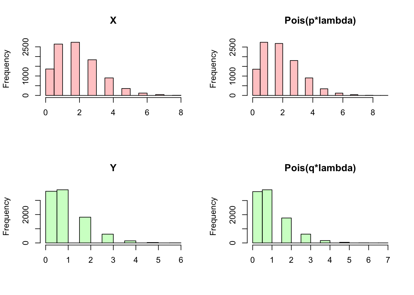
#re-set grid
par(mfrow = c(1,1))

#create a heat-map
#group data, calculate density
data <- data.frame(X, Y)
data = group_by(data, X, Y)
data = summarize(data, density = n())
## `summarise()` has grouped output by 'X'. You can override using the `.groups` argument.data$density = data$density/sims
#plot
ggplot(data = data, aes(X, Y)) +
geom_tile(aes(fill = density), color = "white") +
scale_fill_gradient(low = "white", high= "red", name = "Density") +
ggtitle("Empirical Density of X and Y") +
theme(plot.margin = unit(c(1.8,.5,1.75,1.55), "cm")) +
theme(plot.title = element_text(family = "Trebuchet MS",
color="#383838", face="bold", size=25, vjust = 2)) +
theme(axis.title.x = element_text(family = "Trebuchet MS",
color="#383838", face="bold", size=22, vjust = -1.5),
axis.title.y = element_text(family = "Trebuchet MS",
color="#383838", face="bold", size=22, vjust = 2)) +
theme(axis.text.x = element_text(face="bold", color="#383838",
size=14),
axis.text.y = element_text(face="bold", color="#383838",
size=14))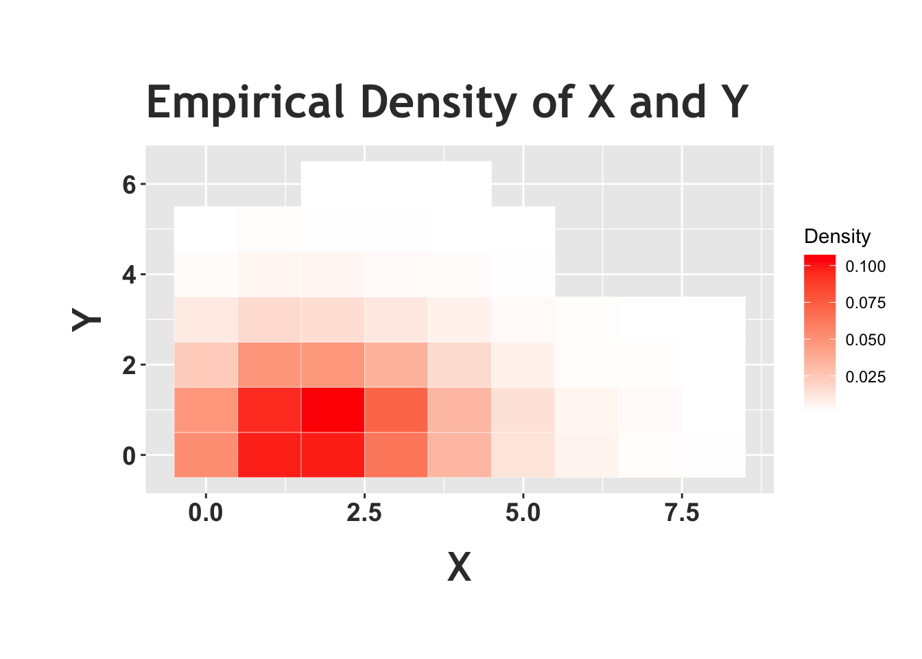
Above we see the empirical heat map of \(X\) and \(Y\) from the Chicken-Egg problem, and we can compare this to the analytical heat map of two independent Poisson random variables below. We see that this heat map looks similar to the one above. The periphery is more filled out in the analytical case; we simply don’t observe these low-probability edges when we run a simulation, but we can plot the probabilities analytically. We can also see here, again, that the relative distributions of the rows (when we condition on specific values of \(Y\)) is similar across rows, again supporting that conditioning on \(Y\) doesn’t change the distribution of \(X\). You could do this same exercise and consider the columns; fix a value of \(X\) and look at the distribution of \(Y\). The implication (which we proved above) is that the random variables are independent.
#recycle  parameters
lambda = 3
p = 2/3

#define the supports/all combinations, up to 10 (beyond 10 has very low probability)
X.a = 0:7
Y.a = 0:7
data = expand.grid(X.a = X.a, Y.a = Y.a)

#calculate density, just the product of Poisson PMFs (use dpois for the Poisson PMF)
data$density = apply(data, 1, function(x)
    dpois(x[1], lambda*p)*dpois(x[2], lambda*(1 - p)))

#remove points with 0 density
data = data[data$density != 0, ]


#generate a heatmap
ggplot(data = data, aes(X.a, Y.a)) +
  geom_tile(aes(fill = density), color = "white") +
  scale_fill_gradient(low = "white", high= "red", name = "Density") +
  ggtitle("Analytical Density of X and Y") +
  theme(plot.margin = unit(c(1.8,.5,1.75,1.55), "cm")) +
  theme(plot.title = element_text(family = "Trebuchet MS",
            color="#383838", face="bold", size=25, vjust = 2)) +
  theme(axis.title.x = element_text(family = "Trebuchet MS",
            color="#383838", face="bold", size=22, vjust = -1.5),
        axis.title.y = element_text(family = "Trebuchet MS",
            color="#383838", face="bold", size=22, vjust = 2)) +
  theme(axis.text.x = element_text(face="bold", color="#383838",
                           size=14),
          axis.text.y = element_text(face="bold", color="#383838",
                           size=14))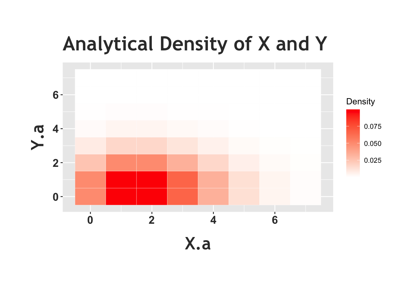
Anyways, the ‘Chicken-Egg’ result is a very interesting (and non-intuitive!) outcome that you surely will see over and over again. It’s important to understand how to prove it, but it’s probably more valuable to remember the final result, so we will restate it one final time. If \(N \sim Pois(\lambda)\), and \(X|N \sim Bin(N,p)\), and \(X + Y = N\), then \(X\) and \(Y\) are independent Poisson random variables with rate parameters \(\lambda p\) and \(\lambda q\), respectively.
Practice
Problems
6.1
Consider a square with area 1 that lies in the first quadrant of the x-y plane, where the bottom left corner starts at the origin (so, \(x\) and \(y\) run from 0 to 1). We pick a random point, \((x,y)\), in this square (the point is chosen uniformly).
Find the joint PDF of \(X\) and \(Y\).
Find the marginal PDF of \(X\).
Find the PDF of \(X\) conditional on \(Y\).
Show that \(X\) and \(Y\) are independent.
6.2
Let \(X \sim N(0, 1)\) and \(Y|X \sim N(X, 1)\). Find the joint PDF of \(X\) and \(Y\).
6.3
You roll a fair, six-sided die \(X\) times, where \(X \sim Pois(\lambda)\). Let \(Y\) be the number of 6’s that you roll. Find \(P(Y > 0\)); you may leave your answer in terms of \(\lambda\).
6.4
There are \(n\) quarters. You flip them all (they are fair) and place them on a table. You then select \(m \leq n\) quarters at random. Let \(X\) be the number of quarters that show heads on the table, and \(Y\) be the number of quarters that show heads that you select. Find the Joint PMF of \(X\) and \(Y\).
6.5
Imagine a standard clock with the hours 1 to 12. The small hand starts at a random hour and moves counterclockwise (i.e., from 4 to 3) or clockwise (i.e., from 10 to 11) with equal probabilities. Let \(X_t\) be the hour that the small hand is at in round \(t\) (i.e., after the hand has moved \(t\) times). Find the joint PMF of \(X_t\) and \(X_{t + 1}\) for \(t \geq 1\).
6.6
Imagine a standard Rubix cube: 6 faces, each with a separate color, each face colored with 9 stickers (for a total of 54 stickers on the cube). You peel off \(n \leq 54\) random stickers. Let \(R\) be the number of red stickers that you get, and \(Y\) be the number of yellow stickers. Find the Joint PMF of \(R\) and \(Y\).
6.7
Let \(X\), \(Y\) and \(Z\) be continuous random variables with the joint PDF given by \(f(x, y, z) = x^2 + y^2 + z^2\), where the support of each random variable is the interval from 0 to 1. Find \(f(x)\), \(f(y)\) and \(f(z)\), and check that they are all valid PDFs.
6.8
Let \(X,Y\) be i.i.d. \(N(0, 1)\). Find \(E\big((X + Y)^2\big)\) using 2-D LoTUS. You can leave your answer as an un-simplified integral.
6.9
CJ is waiting for a bus that has wait time \(X \sim Pois(\lambda_1)\) and a car that has wait time \(Y \sim Expo(\lambda_2)\), where \(X\) and \(Y\) are independent.
In the case where \(\lambda_1 = \lambda_2\), what is the probability that the bus arrives first?
In the case where \(\lambda_1\) and \(\lambda_2\) are not necessarily equal, what is the probability that the bus arrives first? Provide some intuition (i.e., discuss how this answer changes with \(\lambda_1\) and \(\lambda_2\) and say why this is the case).
Now imagine that CJ is also waiting for a plane that has wait time \(Z \sim Pois(\lambda_3)\), independently of \(X\) and \(Y\). What is the probability that this plane arrives first (i.e., before the bus and car), in the general case where the parameters of \(X\), \(Y\) and \(Z\) are not necessarily equal?
6.10
Let \(X \sim N(0, 1)\) and \(Y|X \sim N(x, 1)\). Find \(f(x,y)\).
BH Problems
The problems in this section are taken from Blitzstein and Hwang (2014). The questions are reproduced here, and the analytical solutions are freely available online. Here, we will only consider empirical solutions: answers/approximations to these problems using simulations in R.
BH 7.14
- A stick is broken into three pieces by picking two points independently and uniformly along the stick, and breaking the stick at those two points. What is the probability that the three pieces can be assembled into a triangle?
Hint: A triangle can be formed from 3 line segments of lengths \(a,b,c\) if and only if \(a,b,c \in (0,1/2)\). The probability can be interpreted geometrically as proportional to an area in the plane, avoiding all calculus, but make sure for that approach that the distribution of the random point in the plane is Uniform over some region.
- Three legs are positioned uniformly and independently on the perimeter of a round table. What is the probability that the table will stand?
BH 7.18
Let \((X,Y)\) be a uniformly random point in the triangle in the plane with vertices \((0,0), (0,1), (1,0)\). Find the joint PDF of \(X\) and \(Y\), the marginal PDF of \(X\), and the conditional PDF of \(X\) given \(Y\).
BH 7.19
A random point \((X,Y,Z)\) is chosen uniformly in the ball \(B = \{(x,y,z): x^2 + y^2 + z^2 \leq 1 \}\).
Find the joint PDF of \(X,Y,Z\).
Find the joint PDF of \(X,Y\).
Find an expression for the marginal PDF of \(X\), as an integral.
BH 7.20
Let \(U_1,U_2,U_3\) be i.i.d. Unif(\(0,1\)), and let \(L = \min(U_1,U_2,U_3), M = \max(U_1,U_2,U_3)\).
Find the marginal CDF and marginal PDF of \(M,\) and the joint CDF and joint PDF of \(L,M\).
Find the conditional PDF of \(M\) given \(L\).
BH 7.24
Two students, \(A\) and \(B\), are working independently on homework (not necessarily for the same class). Student \(A\) takes \(Y_1 \sim Expo(\lambda_1)\) hours to finish his or her homework, while \(B\) takes \(Y_2 \sim Expo(\lambda_2)\) hours.
Find the CDF and PDF of \(Y_1/Y_2\), the ratio of their problem-solving times.
Find the probability that \(A\) finishes his or her homework before \(B\) does.
BH 7.26
The bus company from Blissville decides to start service in Blotchville, sensing a promising business opportunity. Meanwhile, Fred has moved back to Blotchville. Now when Fred arrives at the bus stop, either of two independent bus lines may come by (both of which take him home). The Blissville company’s bus arrival times are exactly \(10\) minutes apart, whereas the time from one Blotchville company bus to the next is Expo(\(\frac{1}{10}\)). Fred arrives at a uniformly random time on a certain day.
What is the probability that the Blotchville company bus arrives first? Hint: One good way is to use the continuous law of total probability.
What is the CDF of Fred’s waiting time for a bus?
BH 7.31
Let \(X\) and \(Y\) be i.i.d. \(Unif(0,1)\). Find the standard deviation of the distance between \(X\) and \(Y\).
BH 7.32
Let \(X,Y\) be i.i.d. Expo(\(\lambda\)). Find \(E|X-Y|\) in two different ways: (a) using 2D LOTUS and (b) using the memoryless property without any calculus.
BH 7.59
A \(Pois(\lambda)\) number of people vote in a certain election. Each voter votes for candidate \(A\) with probability \(p\) and for candidate \(B\) with probability \(q=1-p\), independently of all the other voters. Let \(V\) be the difference in votes, defined as the number of votes for \(A\) minus the number for \(B\).
Find \(E(V)\).
Find \(Var(V)\).
BH 7.64
Let \((X_1,\dots,X_k)\) be Multinomial with parameters \(n\) and \((p_1,\dots,p_k)\). Use indicator r.v.s to show that \(Cov(X_i,X_j) = -np_i p_j\) for \(i \neq j\).
BH 7.65
Consider the birthdays of 100 people. Assume people’s birthdays are independent, and the 365 days of the year (exclude the possibility of February 29) are equally likely. Find the covariance and correlation between how many of the people were born on January 1 and how many were born on January 2.
BH 7.67
A group of \(n \geq 2\) people decide to play an exciting game of Rock-Paper-Scissors. As you may recall, Rock smashes Scissors, Scissors cuts Paper, and Paper covers Rock (despite Bart Simpson saying “Good old rock, nothing beats that!”).
Usually this game is played with 2 players, but it can be extended to more players as follows. If exactly 2 of the 3 choices appear when everyone reveals their choice, say \(a,b \in \{\textrm{Rock}, \textrm{Paper}, \textrm{Scissors}\}\) where \(a\) beats \(b\), the game is decisive: the players who chose \(a\) win, and the players who chose \(b\) lose. Otherwise, the game is indecisive and the players play again.
For example, with 5 players, if one player picks Rock, two pick Scissors, and two pick Paper, the round is indecisive and they play again. But if 3 pick Rock and 2 pick Scissors, then the Rock players win and the Scissors players lose the game.
Assume that the \(n\) players independently and randomly choose between Rock, Scissors, and Paper, with equal probabilities. Let \(X, Y , Z\) be the number of players who pick Rock, Scissors, Paper, respectively in one game.
Find the joint PMF of \(X,Y,Z.\)
Find the probability that the game is decisive. Simplify your answer.
What is the probability that the game is decisive for \(n = 5\)? What is the limiting probability that a game is decisive as \(n \to \infty\)? Explain briefly why your answer makes sense.
BH 7.68
Emails arrive in an inbox according to a Poisson process with rate \(\lambda\) (so the number of emails in a time interval of length \(t\) is distributed as \(Pois(\lambda t)\), and the numbers of emails arriving in disjoint time intervals are independent). Let \(X,Y,Z\) be the numbers of emails that arrive from 9 am to noon, noon to 6 pm, and 6 pm to midnight (respectively) on a certain day.
Find the joint PMF of \(X,Y,Z\).
Find the conditional joint PMF of \(X,Y,Z\) given that \(X+Y+Z = 36\).
Find the conditional PMF of \(X+Y\) given that \(X+Y+Z=36\), and find \(E(X+Y|X+Y+Z=36)\) and \(Var(X+Y|X+Y+Z=36)\) (conditional expectation and conditional variance given an event are defined in the same way as expectation and variance, using the conditional distribution given the event in place of the unconditional distribution).