4.6.1 Relative and Expected Rates

When it comes to homophily, there are two ways of measuring the propensity of an actor to associate with those who are the “same” as they are. Relative rates are when actors demonstrate preferences for some groups of actors relative to other groups of actors. Thus, if Ashley has 10 friends in college, seven of which are female and three of which are male, then Ashley seems to prefer having female friends relative to having male friends.

However, what if Ashley goes to a college where there are 700 female students and 300 male students? Would we still think of Ashley as having a preference for female friends? This is the logical behind expected rates. Expected rates are when researchers try to understand with what liklihood an actor would choose a friend at random and then compare that to the observed rate. In this case, at random there is a 70% chance Ashley would choose a female friend and a 30% chance a male friend would be made. Thus, Ashley does not demonstrate a preference for female friends, but actually seems to make friends regardless of gender. If we used a relative rate, we would conclude Ashley prefers female college friends, while under an expected rate, Ashley seems to not care for gender in her friendship decisions.

While it might seem to make more sense to rely on expected rates in research, it is incredibly hard to know what the underlying population of potential associates actually looks like. At the national population level we often have census statistics that could help us know that, if you made a friend at random somewhere in the US, what the odds they would be between 54-65 and female would be. That might not be useful for the specific research question however as people make friends in their communities- schools, clubs, neighborhoods. If you are interested in the case of racial friendship at the neighborhood level, you might not know everyone in the neighborhood. Comparing the observed homophily in respondent’s ego networks might be the best one can do (Ignatow, Poulin, Hunter, and Comeau 2013). Understanding what tools the researcher can access to best examine their question is of critical importance in attainable, as opposed to perfect, research.

4.6.2 EI Homophily Index

The EI homophily index is one of two ways that we will present to think about homophily in an ego-network. The EI homophily index is a relative measure of homophily because it does not consider the underlying population as would be required in an expected rate. Although it might be nice to calculate an expected rate, researchers can often do interesting things even without this data.

The EI homophily index is a measure of in- and out-group preference. One simply subtracts the number of out-group ties from the number of in-group ties, divided by the total number of ties.

\[ \begin{equation} EI=\frac{External-Internal}{External+Internal} \end{equation} \]

Thus, an EI score of -1 means complete homophily- the individual only has relationships with actors of the same “type” as they themselves are. An EI score of 1 means complete heterophily- all the alters are of a different “type” than they themselves are. Finally, an EI score of 0 means that an equal number of alters are of both the same “type” as the ego, and different types.

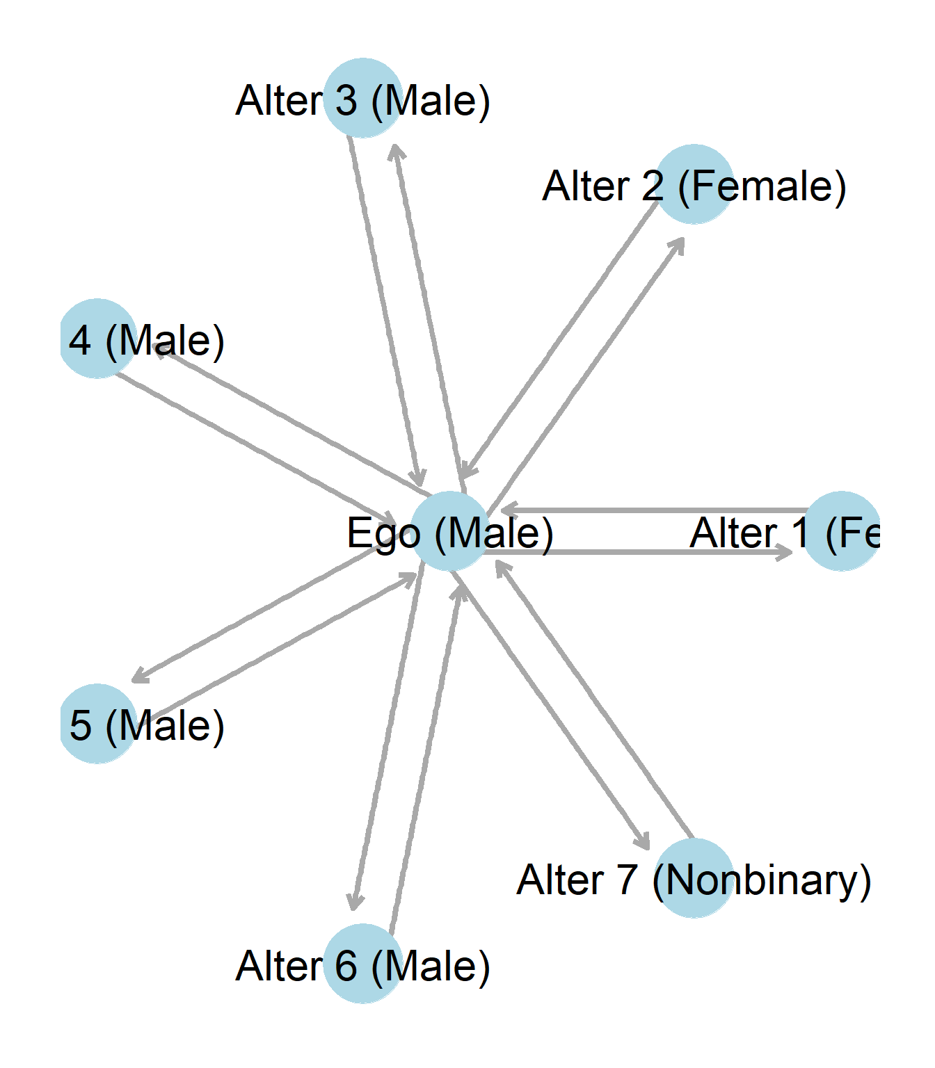
I don’t really know how to fix this messed up graph.

To calculate the EI score for the above ego, we must first ask along what dimension of homophily we are interested in. As discussed above, this must be done to reflect our theoretical question. Let us presume however that we are interested in the relationship between sex and friendship networks. We might ask if the friendship networks of high schoolers are changing over time. If we had older data on friendships, say from 40 years ago, we could compare it with friendship networks from high school students today.

Notice that the ego in this case identifies as male. Notice that ego has four male friends, two female friends, and one non-binary friend. Thus, ego has four friends internal to the same social attribute of interest, and three friends who are not in the same social attribute of interest, regardless of them belonging to different classifications themselves. As such, three (external), minus 4 (internal), over seven total friends, creates an EI homophily score of -1/7, indicating slight homophily.

4.6.3 Blau’s Heterogeneity Index

Blau’s heterogeneity index is a measure of diversity, as opposed to a simple dichotomy of in- or out-group associations as in the case of the EI homophily index. Quite simply, it is the sum of the square of the percentage (p) of the ego’s network belonging to particular groups, subtracted from one.

H Index \[ \begin{equation} H = 1-\sum_{k}p_k^{2} \end{equation} \]

The the H index has a maximum of one, meaning that all of a person’s friends are of the same group as each other. Unlike in the EI homophily index, the ego’s own group membership does not matter. A woman with only male friends would have an H index of 1, just as a woman with only female friends would have an H index of 1. It simply means that there is no diversity in the types of friends the ego has. Conversely, an H index score that approaches towards 0 implies greater heterogeneity, or diversity, in an ego’s network relations.

Solving for the H index of the above ego network presented in the above EI homophily section, is a matter of identifying the different groups in the ego’s network.

\[ \begin{equation} H = 1-\sum{p_{male}^{2}}{p_{female}^{2}}{p_{nonbinary}^{2}} \end{equation} \]

As shown above, the ego’s network has ties to three different groups that we are interested in as this is how many gender identities are in the ego’s network. The next step is to find what percentage of each group makes up the ego’s network. Once this is done, a little bit of math solves for the H index score.

\[ \begin{equation} H = 1-\sum{(\frac{4}{7}_{male}^{2})}+{(\frac{2}{7}_{female}^{2})}+{(\frac{1}{7}_{nonbinary}^{2})}=1-\sum{(.33)}+{(.08)}+{(.02)}=.57 \end{equation} \]

The resulting H index is .57 on a scale of 0 to 1. We might now ask what that means. Remember however that it is mostly useful in comparison to other people’s ego networks. If someone 40 years ago had an H index score of .85, it would mean that the person today has a more diverse ego-network when it comes to the gender of their friends than a high schooler in the past. We can then start to theorize why. Remember however that we would need to do this with a large number of students in the past and today so that we could be comparing true averages. If you’ve taken a statistics class, one can think about sampling ego networks in the same way we sample people’s opinions or their heights. The more we sample, the more we can get closer to finding the average in the population.

4.6.4 Gower and Legendre (1985)

This section is not important for this class

\[ \begin{equation} \sqrt(\frac{a}{(a+b)}-\frac{c}{(c+d)})(\frac{a}{(a+c)}-\frac{b}{(b+c)}) \end{equation} \]