4.2 Degree Centrality
How should we define the idea of centrality? We might imagine that someone “central” to the network is someone who holds some sort of important, advantaged position in the network. The problem is, that there are lots of specific ways we can think of centrality, and thus different ways of mathematically defining the concept.
The first way of defining centrality is simply as a measure of how many alters an ego shares ties with. This simply takes a nodes degree as introduced in Chapter 2, and begins to consider this measure as a reflection of centrality. The logic is that those with more alters, compared to those with fewer, hold a more prominent place in the network.
Equation 1 presents how degree centrality is calculated. Although it might seem a simple task to just add up the number of connections of each node, that is essentially what the below mathematical equation is doing! Mathematical notation plays an important role in expressing network measures in succint formats.
Degree Centrality \[ \begin{equation} C_D(j) = \sum_{j= 1}^{n}A_{ij} \end{equation} \] {\tag{0.2}}
How to Read Equations for Matrix Operations
Depending on your background in math, you may or may not already know how to interpret Equation (???)(eq:degcenteq). Essentially, the number at the bottom of the sigma is where to start. The number at the top of the Sigma symbol (\(\Sigma\)) is where to end. The equation to the left is the operation to be performed. Thus, one reads the Equation (???)(eq:degcenteq) as, starting at row \(j=1\), and ending at the last possible row \(n\) (\(n\) is simply the total number of rows in the matrix, \(n\) means to go to the final value in the matrix), add up all possible values of the cells designated by the row \(i\) and column \(j\) combination in matrix A. Thus, to calculate the degree centrality of each \(i = a, b, c\) in the below matrix, each of the following calculations would be performed.
| a | b | c | |
|---|---|---|---|
| a | - | 1 | 0 |
| b | 1 | - | 1 |
| c | 0 | 1 | - |
\(C_D(a)=aa+ab+ac=1\)
\(C_D(b)=ba+bb+bc=2\)
\(C_D(c)=ca+cb+cb=1\)
In the same way if we had the formula:
\[\begin{align*} C_D(i) = \sum_{j = 1}^{n}A_{ij} \end{align*}\]
Then it would be telling us to sum values of each column \(j\) down each row \(i\):
\(C_D(a)=aa+ba+ca=1\)
\(C_D(b)=ab+bb+cb=2\)
\(C_D(c)=ac+bc+cc=1\)
The sigma notation is useful for summarizing this repetitive process in a simple, condensed form.
The same equation is used to calculate the out-degree centrality for an asymmetric matrix is the same as the equation for degree centrality in a symmetric matrix. However, the general equation to calculate in-degree centrality is reversed, adding down the columns j rather than adding across the columns i.
\[ \begin{equation} C_I(i) = \sum_{i = 1}^{n}A_{ij} \end{equation} \]
Remember the example of a directed graph and corresponding asymmetric matrix from the previous chapters? We can use it to understand in- and out-degree centrality.
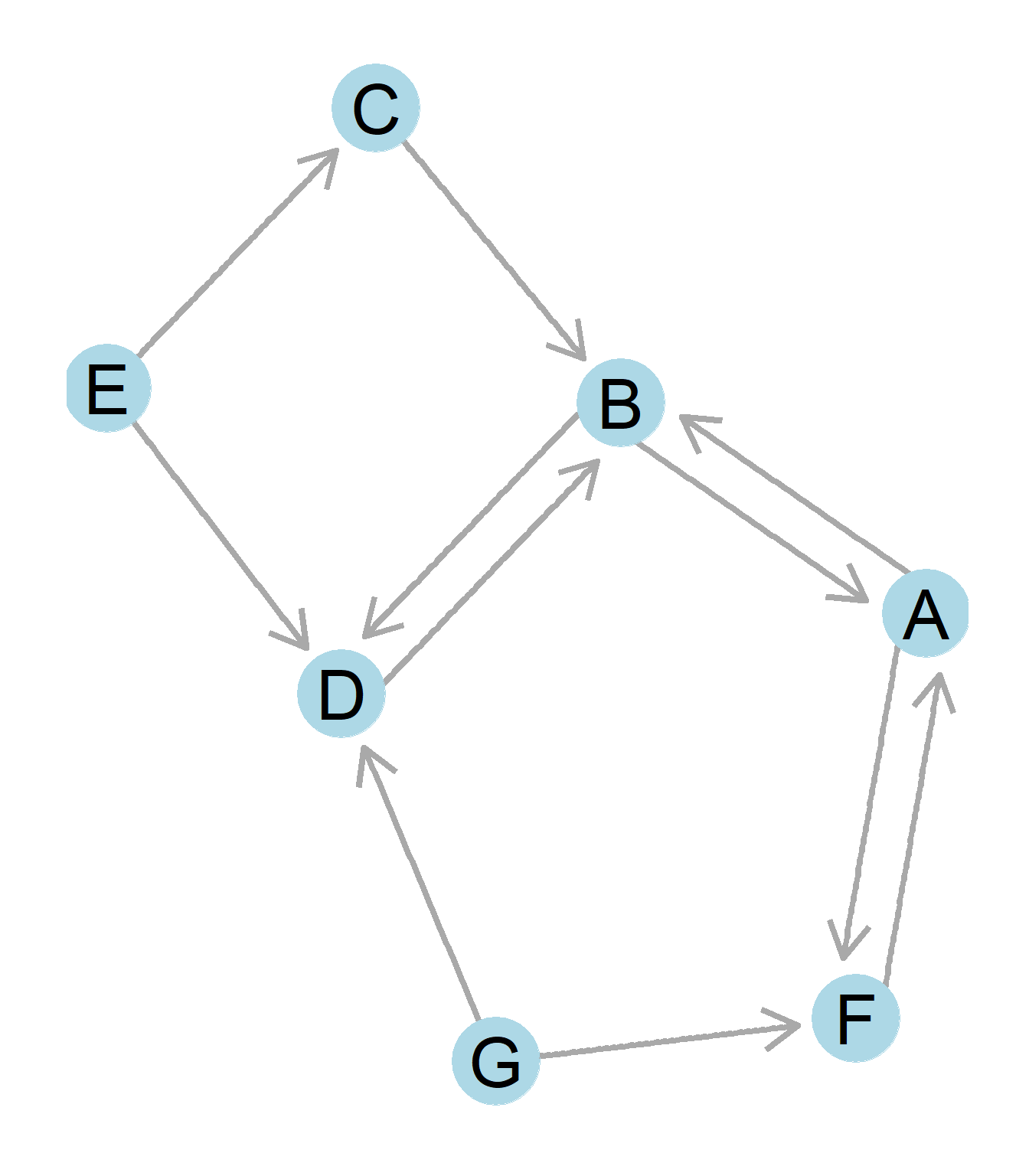 Figure 0.18: A directed graph.
\[ \begin{array}{ccccccccc} & A & B & C & D & E & F & G \\ A & - & 1 & 0 & 0 & 0 & 1 & 0 \\ B & 1 & - & 0 & 1 & 0 & 0 & 0 \\ C & 0 & 1 & - & 0 & 0 & 0 & 0 \\ D & 0 & 1 & 0 & - & 0 & 0 & 0 \\ E & 0 & 0 & 1 & 1 & - & 0 & 0 \\ F & 1 & 0 & 0 & 0 & 0 & - & 0 \\ G & 0 & 0 & 0 & 1 & 0 & 1 & - \\ \end{array} \]
Starting with calculating out-degree, we can look at the matrix. Looking across row A (i), we can see that there are two nodes in the columns (j), which A directs ties to. Thus, the out-degree of node A is two. Likewise, looking down column A (j), we see that A receives ties from two nodes for an in-degree of two. Looking then at the graph, we can confirm that A sends out two ties and receives two ties as well. Doing the same procedure for node G, we would see that adding across the matrix computes that node G sends out two ties, yet adding down the column, G receives no ties, just as a look at the graph would confirm!