4.4 K-Path Centrality

Sade (1989) introduced the idea of k-path centrality. Logically, nodes which are near lots of other nodes, even they are not directly connected, are more closely connected to the network than nodes which are loosely connected through other nodes. It is useful for researchers to be able to examine this easily if their research question calls for measuring this.

K-Path Centrality \[ \begin{equation} C_k(j) = \sum_{j = 1}^{n}A^k_{ij} \end{equation} \]

To do this, we multiply the matrix by itself equivalent to the path length we are interested in solving for. For example, looking for a k-path of k=2 would find all nodes two steps away. To solve, one would simply square the matrix. If you remember from chapter 3, this is the same thing as a reachability matrix! Now, we’ve simply shifted our thinking about it, to realize that it is interpretable as a measure of centrality. With some manipulation of the graph, we can easily calculate how far away a given node is from alters to which they are not directly connected.

Note that k-path centrality is actually a generalization of degree centrality.Note that this formula reduces to equivalence wtih degree centrality for k=1, as k=1 is simply the condition which asks if two nodes are adjacent or not.

Figure 4.1

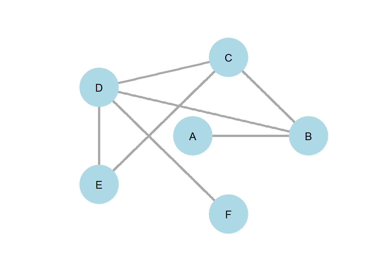Figure 4.1 provides a simple example of how k-path centrality of two provides insights that degree centrality alone fails to provide. Nodes A and F both have a degree centrality of one. However, node F has a 2-path centrality of 3, while node A has a 2-path centrality of 2. We might then think of node F as better connected to the network than node A.