1.3 What p-values would you expect?

This section is based on ideas I learned from homework assignment 1 in Daniel Lakens’s Coursera class Improving your statistical inferences.

What distribution of p-values would you expect if there is a true effect and you repeated the study many times? What if there is no true effect? The answer is completely determined by the statistical power of the study.

To see this, run 100,000 simulations of an experiment measuring the average IQ from a sample of size n = 26. The samples will be 26 random values from the normal distribution centered at 106 with a standard deviation of 15. H0 is \(\mu\) = 100.

# 100,000 random samples of IQ simulations from a normal distribution where
# sigma = 15. True population value is 100, but we'll try other values.
n_sims <- 1E5
mu <- 100
sigma <- 15

run_sim <- function(mu_0 = 106, n = 26) {
  data.frame(i = 1:n_sims) %>%
    mutate(
      x = map(i, ~ rnorm(n = n, mean = mu_0, sd = sigma)),
      z = map(x, ~ t.test(., mu = mu)),
      p = map_dbl(z, ~ .x$p.value),
      x_bar = map_dbl(x, mean)
    ) %>%
    select(x_bar, p)
}

The null hypothesis is that the average IQ is 100. Our rigged simulation finds an average IQ of 106 - an effect size of 6.

sim_106_26 <- run_sim(mu_0 = 106, n = 26)

glimpse(sim_106_26)
## Rows: 100,000
## Columns: 2
## $ x_bar <dbl> 104.0366, 107.4146, 106.3826, 101.9452, 104.9108, 106.0985, 109.…
## $ p     <dbl> 0.1764747839, 0.0345864346, 0.0419669200, 0.4522238256, 0.065089…

mean(sim_106_26$x_bar)
## [1] 106.0062

The statistical power achieved by the simulations is 50%. That is, the typical simulation detected the effect size of 6 at the .05 significance level about 50% of the time.

pwr.t.test(
  n = 26,
  d = (106 - 100) / 15,
  sig.level = .05,
  type = "one.sample",
  alternative = "two.sided"
)

## 
##      One-sample t test power calculation 
## 
##               n = 26
##               d = 0.4
##       sig.level = 0.05
##           power = 0.5004646
##     alternative = two.sided

That means that given a population with an average IQ of 106, a two-sided hypothesis test of H0: \(\mu\) = 100 from a sample of size 26 will measure an \(\bar{x}\) with a p-value under .05 only 50% of the time. You can see that in this histogram of p-values.

sim_106_26 %>% plot_sim()

Had there been no effect to observe, you’d expect all p-values to be equally likely, so the 20 bins would all have been 5% of the number of simulations – i.e., uniformly distributed under the null. This is called “0 power”, although 5% of the p-values will still be significant at the .05 level. The 5% of p-values < .05 is the Type II error rate - that probability of a positive test result when there is no actual effect to observe.

run_sim(mu_0 = 100, n = 26) %>%
  plot_sim(mu_0 = 100)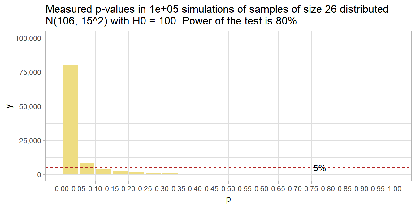

If you want a higher powered study that would detect the effect at least 80% of the time (the normal standard), you’ll need a higher sample size. How high? Conduct the power analysis again, but specify the power while leaving out the sample size.

pwr.t.test(
  power = 0.80,
  d = (106 - 100) / 15,
  sig.level = .05,
  type = "one.sample",
  alternative = "two.sided"
)

## 
##      One-sample t test power calculation 
## 
##               n = 51.00945
##               d = 0.4
##       sig.level = 0.05
##           power = 0.8
##     alternative = two.sided

You need 51 people (technically, you might want to round up to 52). Here’s what that looks like. 80% of p-values are below .05 now.

run_sim(mu_0 = 106, n = 51) %>%
  plot_sim(mu_0 = 106)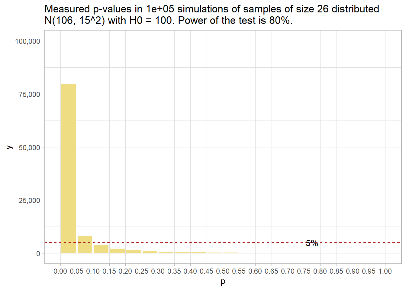

So far, we’ve discovered that when there is an effect, the probability that the measure p-value is under the \(\alpha\) significance level equals the power of the study, 1 - \(\beta\) - the true positive rate, and \(\beta\) will be above the \(\alpha\) level - the false negative rate. We’ve also discovered that when there is no effect, all p-values are equally likely, so \(\alpha\) of them will be below the \(alpha\) level of significance - the false positive rate, and 1 - \(\alpha\) will be above \(\alpha\) - the true negative rate.

It’s not the case that all p-values below 0.05 are support for the alternative hypothesis. If the statistical power is high enough, a p-value just under .05 can be even less likely under the null hypothesis.

run_sim(mu_0 = 108, n = 51)  %>%
    mutate(bin = case_when(p < .01 ~ "0.00 - 0.01",
                         p < .02 ~ "0.01 - 0.02",
                         p < .03 ~ "0.02 - 0.03",
                         p < .04 ~ "0.03 - 0.04",
                         p < .05 ~ "0.04 - 0.05",
                         TRUE ~ "other")
  ) %>%
  janitor::tabyl(bin)

##          bin     n percent
##  0.00 - 0.01 86618 0.86618
##  0.01 - 0.02  5011 0.05011
##  0.02 - 0.03  2353 0.02353
##  0.03 - 0.04  1353 0.01353
##  0.04 - 0.05   887 0.00887
##        other  3778 0.03778

(Recall that under H0, all p-values are equally likely, so each of the percentile bins would contain 1% of p-values.)

In fact, at best, a p-value between .04 and .05 can only be about four times as likely under the alternative hypothesis as the null hypothesis. If your p-value is just under .05, it is at best weak support for the alternative hypothesis.