4.6 One-Sample Poisson Test
If \(X\) is the number of successes in \(n\) (many) trials when the probability of success \(\lambda / n\) is small, then \(X\) is a random variable with a Poisson distribution, and the probability of observing \(X = x\) successes is
\[f(x;\lambda) = \frac{e^{-\lambda} \lambda^x}{x!} \hspace{1cm} x \in (0, 1, ...), \hspace{2mm} \lambda > 0\]
with \(E(X)=\lambda\) and \(Var(X) = \lambda\) where \(\lambda\) is estimated by the sample \(\hat{\lambda}\),
\[\hat{\lambda} = \sum_{i=1}^N x_i / n.\]
Poisson sampling is used to model counts of events that occur randomly over a fixed period of time. You can use the Poisson distribution to perform an exact test on a Poisson random variable.
Example
You are analyzing goal totals from a sample consisting of the 95 matches in the first round of the 2002 World Cup. The average match produced a mean/sd of 1.38 \(\pm\) 1.28 goals, lower than the 1.5 historical average. Should you reject the null hypothesis that the sample is representative of typical values?
Conditions
- The events must be independent of each other. In this case, the goal-count in one match has no effect on goal-counts in other matches.
- The expected value of each event must be the same (homogeneity). In this case, the expected goal-count of each match is the same regardless of which teams are playing. This assumption is often dubious, causing the distribution variance to be larger than the mean, a conditional called over-dispersion.
You might also check whether the data is consistent with a Poisson model. This is random sampling, but the data violates the \(\ge\) 5 rule because the minimum expected frequency was 0. To comply with the minimum frequency rule, lump the last six categories into “3-8”.
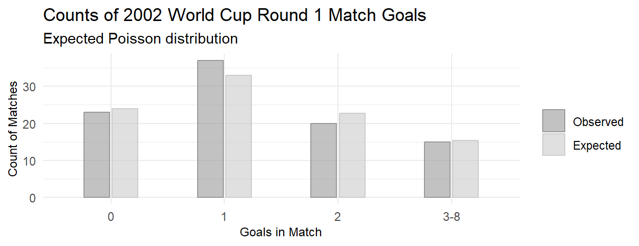
The minimum expected frequency was 15, so now the chi-squared test of independence is valid. Compare the expected values to the observed values with the chi-squared goodness of fit test, but in this case \(df = 4 - 1 - 1\) because the estimated parameter \(\lambda\) reduces the df by 1. You cannot set df in chisq.test(), so perform the test manually.
(X2 <- sum((o - e)^2 / e))
## [1] 0.8618219
(p.value <- pchisq(q = X2, df = length(j) - 1 - 1, lower.tail = FALSE))
## [1] 0.6499168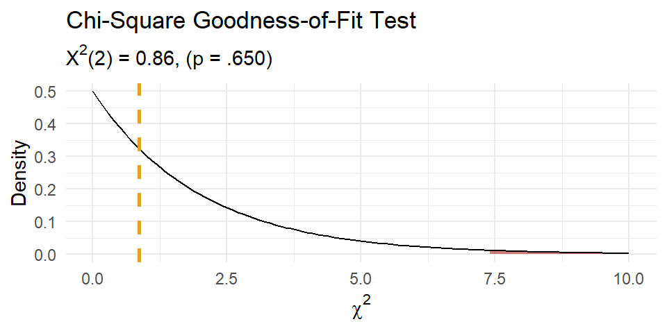
Of the 95 World Cup matches, 23 had no goals, 37 had one goal, 20 had two goals, and 15 had 3-8 goals. A chi-square goodness-of-fit test was conducted to determine whether the observed goal counts follow a Poisson distribution. The minimum expected frequency was 15. The chi-square goodness-of-fit test indicated that the number of goals scored was not statistically significantly different from the frequencies expected from a Poisson distribution (\(X^2\)(2) = 0.862, p = 0.650).
Results
The conditions for the exact Poisson test were met, so go ahead and run the test.
(pois_val <- poisson.test(
  x = sum(dat_pois$goals * dat_pois$freq),
  T = sum(dat_pois$freq),
  r = 1.5)
)
##
## Exact Poisson test
##
## data: sum(dat_pois$goals * dat_pois$freq) time base: sum(dat_pois$freq)
## number of events = 131, time base = 95, p-value = 0.3567
## alternative hypothesis: true event rate is not equal to 1.5
## 95 percent confidence interval:
## 1.152935 1.636315
## sample estimates:
## event rate
## 1.378947Construct a plot showing the 95% CI around the hypothesized value. For a Poisson distribution, I built the distribution around the expected value, \(n\lambda\), not the rate, \(\lambda\).
I think you could report these results like this.
A one-sample exact Poisson test was run to determine whether the number of goals scored in the first round of the 2002 World Cup was different from past World Cups, 1.5. A chi-square goodness-of-fit test indicated that the number of goals was not statistically significantly different from the counts expected in the Poisson distribution (\(X^2\)(2) = 0.862, p = 0.650). Data are mean \(\pm\) standard deviation, unless otherwise stated. Mean goals scored (1.38 \(\pm\) 1.28) was lower than the historical mean of 1.50, but was not statistically significantly different (95% CI, 1.15 to 1.64), p = 0.357.