6.4 Case Study: Pearson, Spearman, Kendall
This case study works with two data sets. dat1 is composed of two continuous variables; dat2 is composed of two ordinal variables.
A researcher investigates the relationship between cholesterol concentration and time spent watching TV, time_tv, in n = 100 otherwise healthy 45 to 65 year old men (dat1). This data set will meet the conditions for Pearson, so we try all three tests on it.
A researcher investigates the relationship between the level of agreement with the statement “Taxes are too high” (tax_too_high, four level ordinal) and participant income level (three level ordinal) (dat2). The ordinal variables rule out Pearson, leaving Spearman and Kendall.
Conditions
Pearson’s correlation applies when X and Y are continuous (interval or ratio) paired variables with 1) a linear relationship that 2) has no significant outliers, and 3) are bivariate normal. Spearman’s rho and Kendall’s tau only require that X and Y be at least ordinal with 1) a monotonically increasing or decreasing relationship.
- Linearity and Monotonicity. A visual inspection of a scatterplot should find a linear relationship (Pearson) or monotonic relationship (Spearman and Kendall).
Pearson’s correlation additionall requires
- No Outliers. Identify outliers with the scatterplot.
- Normality. Bivariate normality is difficult to assess. Instead, check that each variable is individually normally distributed. Use the Shapiro-Wilk test.
Linearity / Monotonicity
Assess linearity and monotonicity with a scatter plot. dat1 is plotted on the left in Figure 6.1. A second version that fails the linearity test is shown to the right. If the linear relationship assumption fails, consider transforming the variable instead of reverting to Spearman or Kendall.
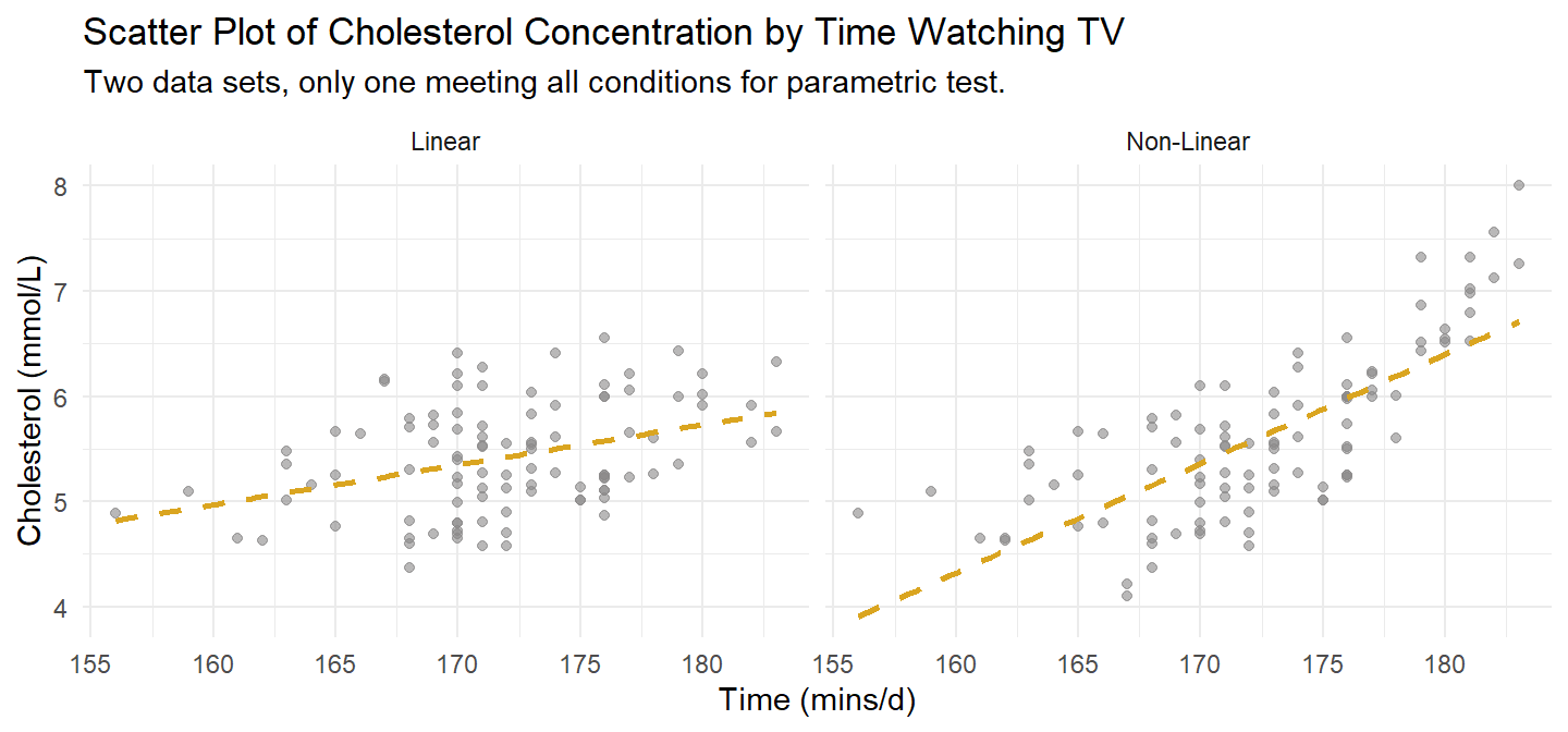
Figure 6.1: The left scatter plot is dat1. It meets Pearson’s linearity condition. A second version at right illustrates what a failure might look like.
The ordinal variable data set dat2 is plotted in Figure 6.2.
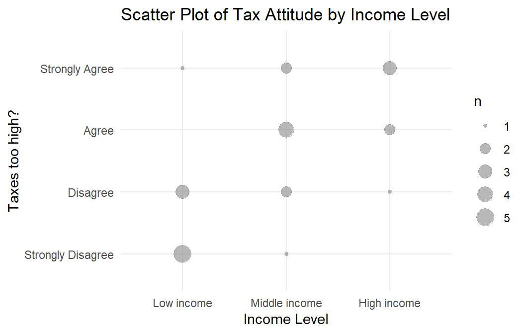
Figure 6.2: dat2 meets the mononicity assumption for Spearman’s rho and Kendall’s tau.
No Outliers
Pearson’s correlation requires no outliers. Both plots in Figure 6.1 are free of outliers. If there were outliers, check whether they are data entry errors or measurement errors and fix or discard them. If the outliers are genuine, leave them in if they do not affect the conclusion. You can also try tranforming the variable. Failing all that, revert to the Spearman’s rho or Kendall’s tau.
Bivariate Normality
Bivariate normality is difficult to assess. If two variables are bivariate normal, they will each be individually normal as well. That’s the best you can hope to check for. Use the Shapiro-Wilk test.
shapiro.test(cs$dat1$time_tv)
##
##  Shapiro-Wilk normality test
##
## data:  cs$dat1$time_tv
## W = 0.97989, p-value = 0.1304
shapiro.test(cs$dat1$cholesterol)
##
##  Shapiro-Wilk normality test
##
## data:  cs$dat1$cholesterol
## W = 0.97594, p-value = 0.06387
If a variable is not normally distributed, you can transform it, carry on regardless since the Pearson correlation is fairly robust to deviations from normality, or revert to Spearman and Kendall.
Test
Calculate Pearson’s correlation, Spearman’s rho, or Kendall’s tau. dat meets the assumptions for Pearson’s correlation, but try Spearman’s rho and Kendall’s tau too, just to see how close they come to Pearson. dat2 only meets the assumptions for Spearman and Kendall.
Pearson’s Correlation
dat1 met the conditions for Pearson’s correlation.
(cs$cc_pearson <-
  cor.test(cs$dat1$cholesterol, cs$dat1$time_tv, method = "pearson")
)
##
## Pearson's product-moment correlation
##
## data: cs$dat1$cholesterol and cs$dat1$time_tv
## t = 3.9542, df = 98, p-value = 0.0001451
## alternative hypothesis: true correlation is not equal to 0
## 95 percent confidence interval:
## 0.1882387 0.5288295
## sample estimates:
## cor
## 0.3709418r = 0.37 falls in the range of a “moderate” linear relationship. \(r^2\) = 14% is the coefficient of determination. Interpret it as the percent of variability in one variable that is explained by the other. If you are not testing a hypothesis (HO: \(\rho \ne 0\)), you can report just report r. Otherwise, include the p-value. Report your results like this:
A Pearson’s product-moment correlation was run to assess the relationship between cholesterol concentration and daily time spent watching TV in males aged 45 to 65 years. One hundred participants were recruited.
Preliminary analyses showed the relationship to be linear with both variables normally distributed, as assessed by Shapiro-Wilk’s test (p > .05), and there were no outliers.
There was a statistically significant, moderate positive correlation between daily time spent watching TV and cholesterol concentration, r(98) = 0.37, p < .0005, with time spent watching TV explaining 14% of the variation in cholesterol concentration.
You wouldn’t use Spearman’s rho or Kendall’s tau here since the more precise Pearson’s correlation is available. But just out of curiosity, here are the correlations using those two measures.
cor(cs$dat1$cholesterol, cs$dat1$time_tv, method = "kendall")
## [1] 0.2383971
cor(cs$dat1$cholesterol, cs$dat1$time_tv, method = "spearman")
## [1] 0.3322122
Both Kendall and Spearman produced more conservative estimates of the strength of the relationship - Kendall especially so.
You probably wouldn’t use linear regression here either because it describes the linear relationship between a response variable and changes to an independent explanatory variable. Even though we are reluctant to interpret a regression model in terms of causality, that is what is implied the formulation y ~ x and independence assumption in of X. Nevertheless, correlation and regression are related. The slope term in a simple linear regression of the normalized values equals the Pearson correlation.
lm(
  y ~ x,
  data = cs$dat1 %>% mutate(y = scale(cholesterol), x = scale(time_tv))
)
##
## Call:
## lm(formula = y ~ x, data = cs$dat1 %>% mutate(y = scale(cholesterol),
## x = scale(time_tv)))
##
## Coefficients:
## (Intercept) x
## -3.092e-16 3.709e-01Spearman’s Rho
Data set dat2 did not meet the conditions for Pearson’s correlation, so use Spearman’s rho and/or Kendall’s tau.
Start with Spearman’s rho. Recall that Spearman’s rho is just the Pearson correlation applied to the ranks. Recall also that the Pearson’s correlation is just the covariance divided by the product of the standard deviations. You can quickly calculate it by hand.
cov(rank(cs$dat2$income), rank(cs$dat2$tax_too_high)) /
  (sd(rank(cs$dat2$income)) * sd(rank(cs$dat2$tax_too_high)))
## [1] 0.6024641Use the function though. I don’t get why cor.test requires x and y be numeric.
(cs$spearman <-
  cor.test(
    as.numeric(cs$dat2$tax_too_high),
    as.numeric(cs$dat2$income),
    method = "spearman")
)
## Warning in cor.test.default(as.numeric(cs$dat2$tax_too_high),
## as.numeric(cs$dat2$income), : Cannot compute exact p-value with ties##
## Spearman's rank correlation rho
##
## data: as.numeric(cs$dat2$tax_too_high) and as.numeric(cs$dat2$income)
## S = 914.33, p-value = 0.001837
## alternative hypothesis: true rho is not equal to 0
## sample estimates:
## rho
## 0.6024641Interpret the statistic using the same rule of thumb as for Pearson’s correlation. A rho over .5 is a strong correlation.
A Spearman’s rank-order correlation was run to assess the relationship between income level and views towards income taxes in 24 participants. Preliminary analysis showed the relationship to be monotonic, as assessed by visual inspection of a scatterplot. There was a statistically significant, strong positive correlation between income level and views towards income taxes, \(r_s\) = 0.602, p = 0.002.
Kendall’s Tau
Recall that Kendall’s tau is a function of concordant (C), discordant (D) and tied (Tx and Ty) pairs of observations. The manual calculation is a little more involved. Here is the function instead.
(cs$kendall <-
  cor.test(
    as.numeric(cs$dat2$tax_too_high),
    as.numeric(cs$dat2$income),
    method = "kendall")
)
## Warning in cor.test.default(as.numeric(cs$dat2$tax_too_high),
## as.numeric(cs$dat2$income), : Cannot compute exact p-value with ties##
## Kendall's rank correlation tau
##
## data: as.numeric(cs$dat2$tax_too_high) and as.numeric(cs$dat2$income)
## z = 2.9686, p-value = 0.002991
## alternative hypothesis: true tau is not equal to 0
## sample estimates:
## tau
## 0.5345225As with the case study on cholesterol and television, Kendall’s tau was more conservative than Spearman’s rho. \(\tau_b\) = 0.535 is still in the “strong” range, though just barely.
A Kendall’s tau-b correlation was run to assess the relationship between income level and views towards income taxes amongst 24 participants. Preliminary analysis showed the relationship to be monotonic, as assessed by visual inspection of a scatterplot. There was a statistically significant, strong positive correlation between income level and the view that taxes were too high, \(\tau_b\) = 0.535, p = 0.003.