4.1 One-Sample Mean z Test

The z test is also called the normal approximation z test. It only applies when the sampling distribution of the population mean is normally distributed with known variance, and there are no significant outliers. The sampling distribution is normally distributed when the underlying population is normally distributed, or when the sample size is large \((n >= 30)\), as follows from the central limit theorem. The t test returns similar results, plus it is valid when the variance is unknown, and that is pretty much always. For that reason, you probably will never use this test.

Under the normal approximation method, the measured mean \(\bar{x}\) approximates the population mean \(\mu\), and the sampling distribution has a normal distribution centered at \(\mu\) with standard error \(se_\mu = \frac{\sigma}{\sqrt{n}}\) where \(\sigma\) is the standard deviation of the underlying population. Define a \((1 - \alpha)\%\) confidence interval as \(\bar{x} \pm z_{(1 - \alpha) {/} 2} se_\mu\), or test \(H_0: \mu = \mu_0\) with test statistic \(Z = \frac{\bar{x} - \mu_0}{se_\mu}\).

Example

The mtcars data set is a sample of n = 32 cars. The mean fuel economy is \(\bar{x} \pm s\) = 20.1 \(\pm\) 6.0 mpg. The prior measured overall fuel economy for vehicles was \(\mu_0 \pm \sigma\) = 18.0 \(\pm\) 6.0 mpg. Has fuel economy improved?

The sample size is \(\ge\) 30, so the sampling distribution of the population mean is normally distributed. The population variance is known, so use the z test.

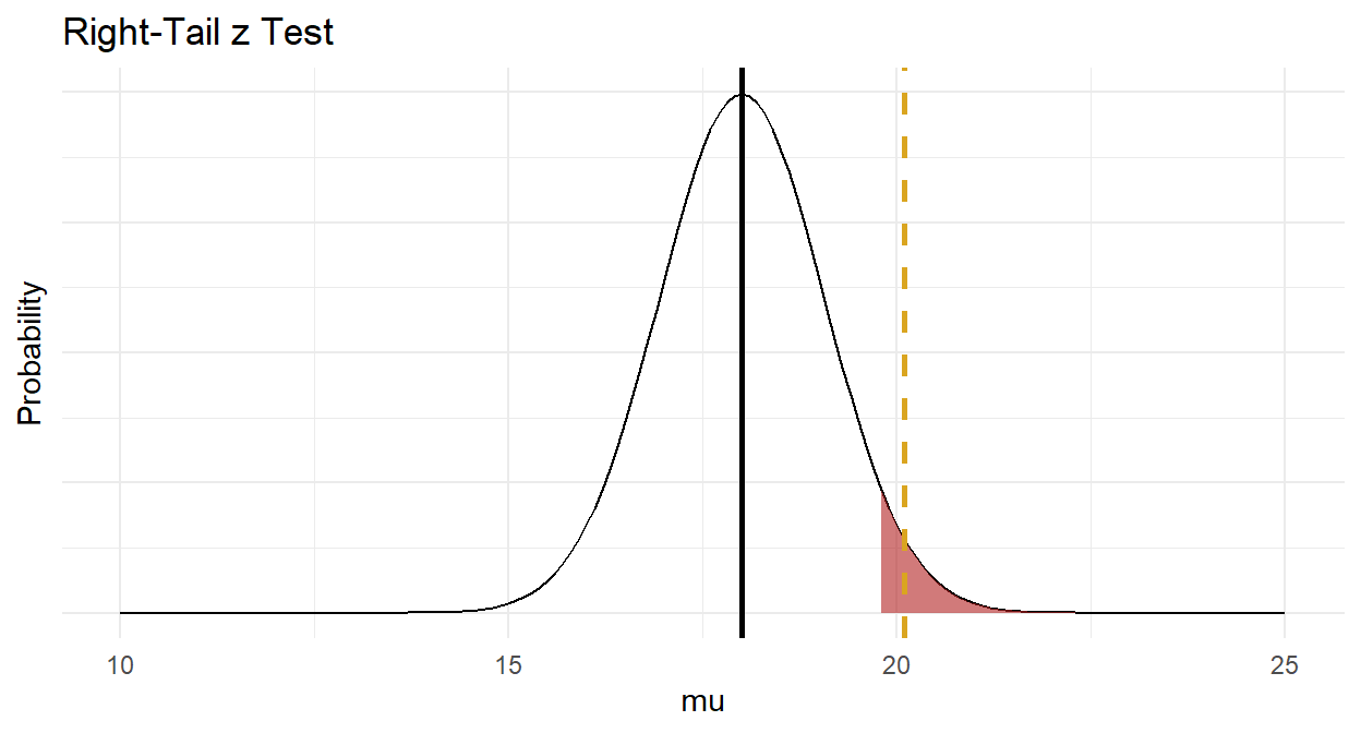
\(H_0: \mu = 16.0\), and \(H_a: \mu > 16.0\) - a right-tail test. The test statistic is \(Z = \frac{\bar{x} - \mu_0}{se_\mu}=\) 1.97 where \(se_{\mu_0} = \frac{\mu_0}{\sqrt{n}} =\) 1.06. \(P(z > Z) =\) 0.0244, so reject \(H_0\) at the \(\alpha =\) 0.05 level of significance.

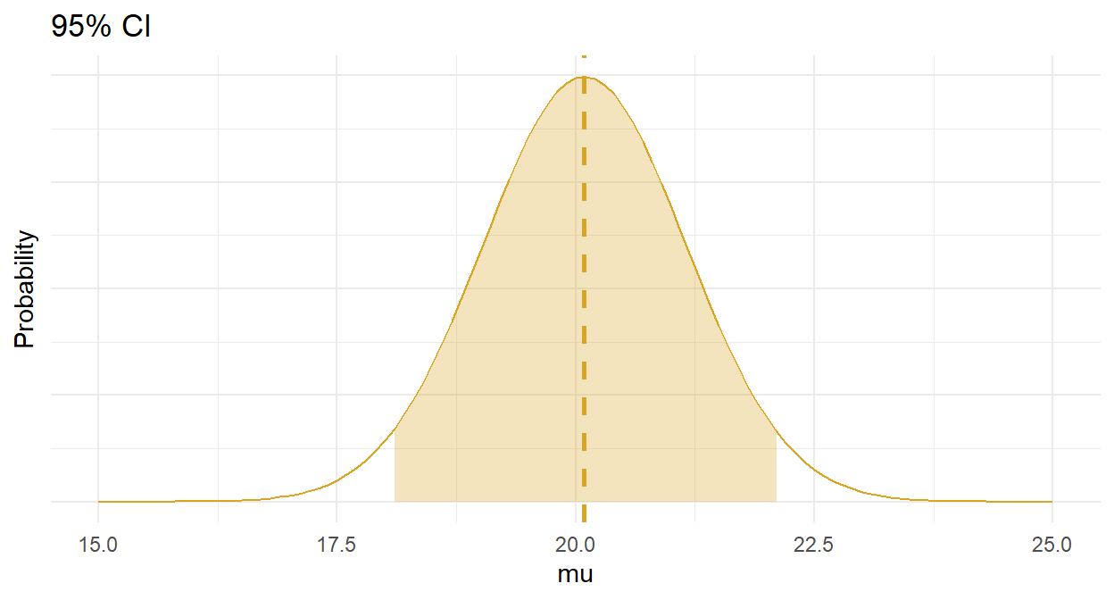
The 95% confidence interval for \(\mu\) is \(\bar{x} \pm z_{(1 - \alpha){/}2} se_\mu\) where \(z_{(1 - \alpha){/}2} =\) 1.96. \(\mu =\) 20.09 \(\pm\) 2.08 (95% CI 18.01 to 22.17).