4.8 One-Sample Proportion z Test

The z-test uses the sample proportion of group \(j\), \(p_j\), as an estimate of the population proportion \(\pi_j\) to evaluate an hypothesized population proportion \(\pi_{0j}\) and/or construct a \((1−\alpha)\%\) confidence interval around \(p_j\) to estimate \(\pi_j\) within a margin of error \(\epsilon\).

The z-test is intuitive to learn, but it only applies when the central limit theorem conditions hold:

the sample is independently drawn, meaning random assignment (experiments), or random sampling without replacement from <10% of the population (observational studies),
there are at least 5 successes and 5 failures,
the sample size is >=30, and
the expected probability of success is not extreme, between 0.2 and 0.8.

If these conditions hold, the sampling distribution of \(\pi\) is normally distributed around \(p\) with standard error \(se_p = \frac{s_p}{\sqrt{n}} = \frac{\sqrt{p(1−p)}}{\sqrt{n}}\). The measured values \(p\) and \(s_p\) approximate the population values \(\pi\) and \(\sigma_\pi\). You can define a \((1 − \alpha)\%\) confidence interval as \(p \pm z_{\alpha / 2}se_p\). Test the hypothesis of \(\pi = \pi_0\) with test statistic \(z = \frac{p − \pi_0}{se_{\pi_0}}\) where \(se_{\pi_0} = \frac{s_{\pi_0}}{\sqrt{n}} = \frac{\sqrt{{\pi_0}(1−{\pi_0})}}{\sqrt{n}}\).

Example

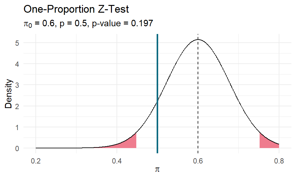
A machine is supposed to randomly churn out prizes in 60% of boxes. In a random sample of n = 40 boxes there are prizes in 20 boxes. Is the machine flawed?

prop.test(20, 40, 0.6, "two.sided", correct = FALSE)

## 
##  1-sample proportions test without continuity correction
## 
## data:  20 out of 40, null probability 0.6
## X-squared = 1.6667, df = 1, p-value = 0.1967
## alternative hypothesis: true p is not equal to 0.6
## 95 percent confidence interval:
##  0.3519953 0.6480047
## sample estimates:
##   p 
## 0.5

The first thing you’ll notice is that prop.test() performs a chi-squared goodness-of-fit test, not a one-proportion Z-test!

chisq.test(c(20, 40-20), p = c(.6, .4), correct = FALSE)

## 
##  Chi-squared test for given probabilities
## 
## data:  c(20, 40 - 20)
## X-squared = 1.6667, df = 1, p-value = 0.1967

It turns out \(P(\chi^2 > X^2)\) equals \(2 \cdot P(Z > z).\) Here is the manual calculation of the chi-squared test statistic \(X^2\) and resulting p-value on 1 dof.

pi_0 <- .6
p <- 20 / 40

observed <- c(p, 1-p) * 40
expected <- c(pi_0, 1-pi_0) * 40

X2 <- sum((observed - expected)^2 / expected)
pchisq(X2, 1, lower.tail = FALSE)

## [1] 0.1967056

And here is the manual calculation of the Z-test statistic \(z\) and resulting p-value.

se <- sqrt(pi_0*(1-pi_0)) / sqrt(40)
z <- (p - pi_0) / se
pnorm(z, lower.tail = TRUE) * 2

## [1] 0.1967056

The 95% CI presented by prop.test() is also not the \(p \pm z_{\alpha / 2}se_p\) Wald interval; it is the Wilson interval!

DescTools::BinomCI(20, 40, method = "wilson")

##      est    lwr.ci    upr.ci
## [1,] 0.5 0.3519953 0.6480047

There are a lot of methods (see ?DescTools::BinomCI), and Wilson is the one Agresti-Coull recommends. If you want Wald, use DescTools::BinomCI() with method = "wald".

DescTools::BinomCI(20, 40, method = "wald")

##      est    lwr.ci    upr.ci
## [1,] 0.5 0.3450512 0.6549488

This matches the manual calculation below.

z_crit = qnorm(1 - .05/2)
se <- sqrt(p*(1-p)) / sqrt(40)

(CI <- c(p - z_crit*se, p + z_crit*se))

## [1] 0.3450512 0.6549488

prop.test() (and chissq.test()) reported a p-value of 0.1967056, so you cannot reject the null hypothesis that \(\pi = 0.6\). It’s good practice to plot this out to make sure your head is on straight.

Incidentally, if you have a margin of error requirement, you can back into the required sample size to achieve it. Just solve the margin of error equation \(\epsilon = z_{\alpha/2}^2 = \sqrt{\frac{\pi_0(1-\pi_0)}{n}}\) for \(n = \frac{z_{\alpha/2}^2 \pi_0(1-\pi_0)}{\epsilon^2}.\)