3.3 Discrete Cases

Suppose you have a string of numbers \([1,1,1,1,0,0,1,1,1,0]\) (7 ones and 3 zeros) produced by a Bernoulli random number generator. What parameter \(p\) was used in the Bernoulli function?²

D <- c(1, 1, 1, 1, 0, 0, 1, 1, 1, 0)

Your best guess is \(p = 0.7\), but how confident are you? Posit eleven competing priors, \(\theta = [.0, .1, \ldots, 1]\) with equal prior probabilities, \(P(\theta) = [1/11, \ldots]\).

theta <- seq(0, 1, by = 0.1)
prior <- rep(1/11, 11)

Using a Bernoulli generative model, the likelihood of observing 7 ones and 3 zeros are \(P(D|\theta) = \theta^7 + (1-\theta)^3.\)

likelihood <- theta^7 * (1 - theta)^3

data.frame(theta, likelihood) %>% 
  ggplot() +
  geom_segment(aes(x = theta, xend = theta, y = 0, yend = likelihood), 
               linetype = 2, color = "steelblue") +
  geom_point(aes(x = theta, y = likelihood), color = "steelblue", size = 3) +
  scale_x_continuous(breaks = theta) +
  theme_minimal() +
  theme(panel.grid.minor = element_blank()) +
  labs(title = expression(paste("Maximum likelihood of observing D is at ", theta, " = 0.7.")),
       x = expression(theta), y = expression(f[theta](D)))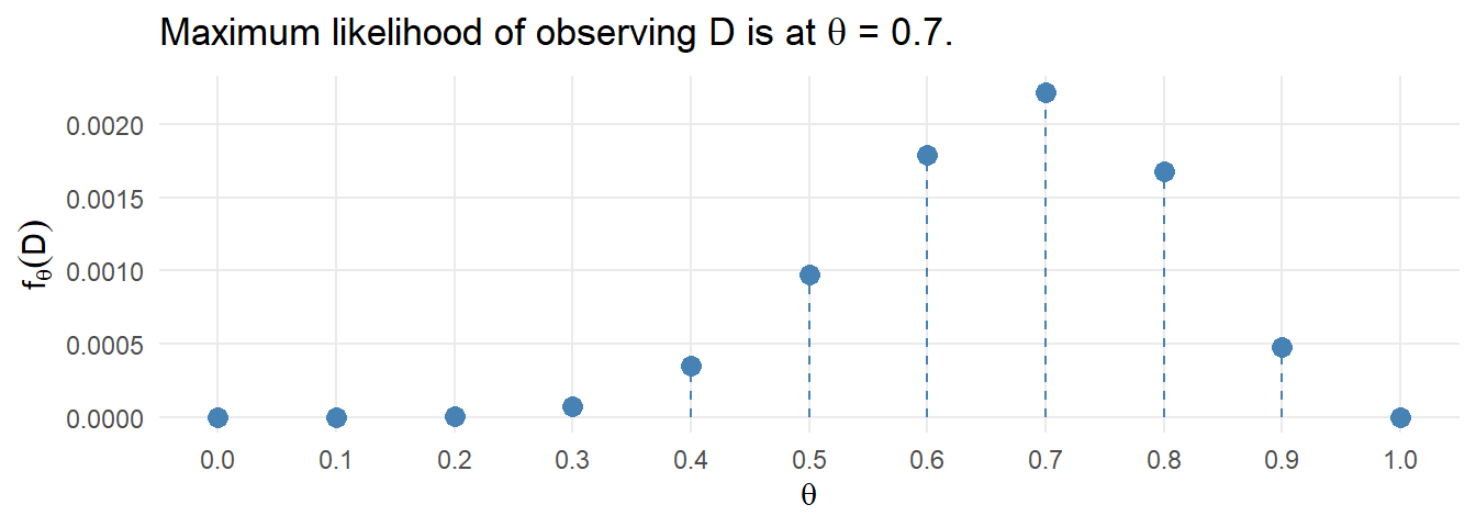

The posterior probability is the likelihood divided by the marginal probability of observing \(D\) multiplied by the prior, \(P(\theta|D) = \frac{P(D|\theta)}{P(D)}\cdot P(\theta).\) In this case, the marginal probability is straight-forward to calculate: it is the sum-product of the priors and their associated likelihoods.

posterior <- likelihood / sum(likelihood * prior) * prior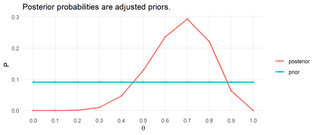

What would the posterior look like if we started with an educated guess on \(P(\theta)\) that more heavily weights \(\theta = 0.7\)?

prior <- c(.05, .05, .05, .05, .05, .10, .15, .20, .15, .10, .05)
posterior <- likelihood / sum(likelihood * prior) * prior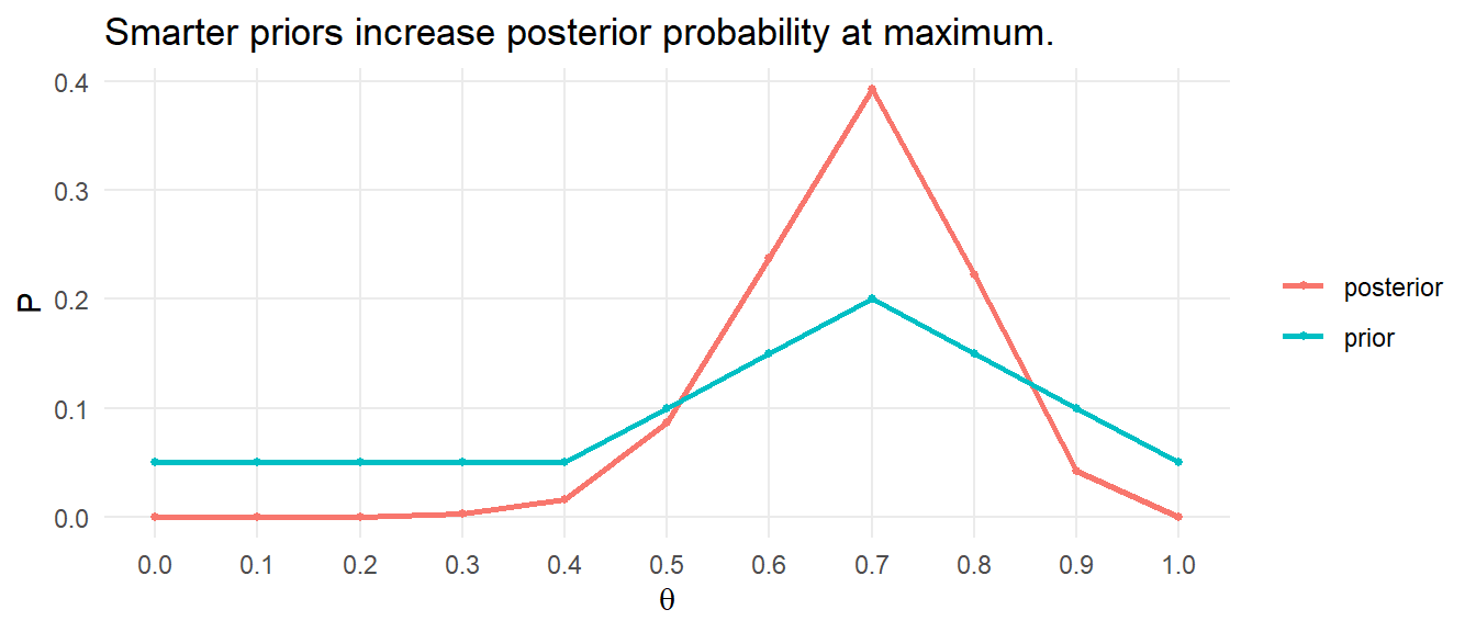

What if we now employ a larger data set? To see, generate a sample of 100 Bernoulli(.7) observations.

D100 <- rbernoulli(100, p = 0.7) %>% as.numeric()

## Warning: `rbernoulli()` was deprecated in purrr 1.0.0.

likelihood <- theta^sum(D100) * (1 - theta)^(length(D100)-sum(D100))
posterior <- likelihood / sum(likelihood * prior) * prior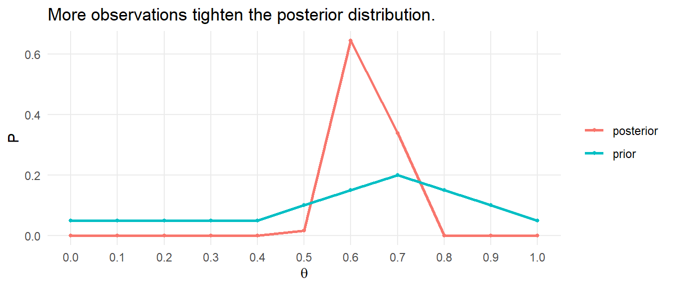

What would it look like if it also had more competing hypotheses, \(\theta \in (0, .01, .02, \ldots, 1)\).

theta <- seq(0, 1, by = .01)
prior <- rep(1/100, 101)
likelihood <- theta^sum(D100) * (1 - theta)^(length(D100)-sum(D100))
posterior <- likelihood / sum(likelihood * prior) * prior

---

2. Example borrowed from chris’ sandbox↩︎