Chapter 2 Likelihood Statistics

Likelihood functions are an approach to statistical inference (along with Frequentist and Bayesian). Likelihoods are functions of a data distribution parameter. For example, the binomial likelihood function is

\[L(\theta) = \frac{n!}{x!(n-x)!}\cdot \theta^x \cdot (1-\theta)^{n-x}\]

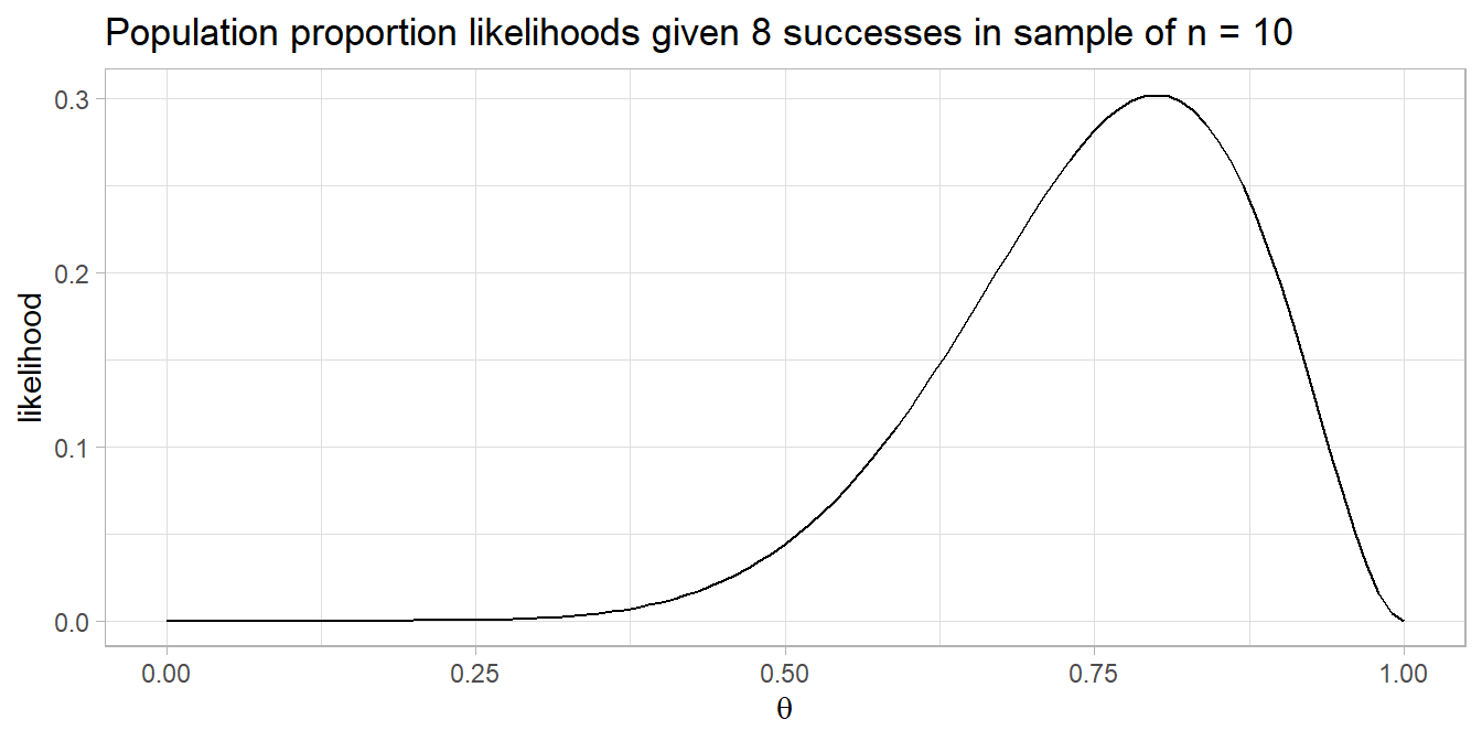
You can use the binomial likelihood function to assess the likelihoods of various hypothesized population probabilities, \(\theta\). Suppose you sample n = 10 coin flips and observe x = 8 successful events (heads) for an estimated heads probability of .8. The likelihood of a fair coin, \(\theta\) = .05 given the evidence is only 0.044.

dbinom(8, 10, .5)

## [1] 0.04394531

You can see from the plot below that the likelihood function is maximized at \(\theta\) = 0.8 (likelihood = 0.302). The actual value of the likelihood is unimportant - it’s a density.

You can combine likelihood estimates by multiplying them. Suppose one experiment finds 4 of 10 heads and a second experiment finds 8 of 10 heads. You’d hope two experiments could be combined to achieve the same result as a single experiment with 12 of 20 heads, and that is indeed the case.

x <- dbinom(4, 10, seq(0, 1, .1))
y <- dbinom(8, 10, seq(0, 1, .1))
z <- dbinom(12, 20, seq(0, 1, .1))

round((x / max(x)) * (y / max(y)), 3)
##  [1] 0.000 0.000 0.000 0.004 0.035 0.119 0.178 0.113 0.022 0.000 0.000
round(z, 3)
##  [1] 0.000 0.000 0.000 0.004 0.035 0.120 0.180 0.114 0.022 0.000 0.000

Compare competing estimates of \(\theta\) with the likelihood ratio. The likelihood of \(\theta\) = .8 vs \(\theta\) = .5 (fair coin) is \(\frac{L(\theta = 0.8)}{L(\theta = 0.5)}\) = 6.87.

A likelihood ratio of >= 8 is moderately strong evidence for an alternative hypothesis. A likelihood ratio of >= 32 is strong evidence for the alternative hypothesis. Keep in mind that likelihood ratios are relative evidence of H1 vs H0 - both hypotheses may be quite unlikely!

A set of studies usually include both positive and negative test results. You can see this from the likelihood plots below. These are the likelihood curves produced from x = [0..3] successes in a sample of 3. Think of this as the likelihood of [0..3] positive findings in 3 studies based on an \(\alpha\) = .05 level of significance and a .80 1 - \(\beta\) statistical power of the study.

The yellow line at .05 is the likelihood of a Type I error of concluding there is an effect when H1 is false. The yellow line at .80 is the likelihood of a Type II error of concluding there is no effect when H1 is true. The likelihood of 0 of 3 experiments reporting a positive effect under \(\alpha\) = .05, 1 - \(\beta\) = .80 is much higher under H0 (\(\theta\) = .05) than under H1 (\(\theta\) = .80): 0.857 vs 0.008 for a likelihood ratio of 107. The likelihood of 1 of 3 experiments reporting a positive effect is still higher under H0 than under H1: 0.135 vs 0.096 for a likelihood ratio of 1.41. For 2 of 3 experiments reporting a positive effect the likelihood ratio is 0.019, and for 3 of 3 experiments reporting a positive effect the likelihood ratio is 0.00024.

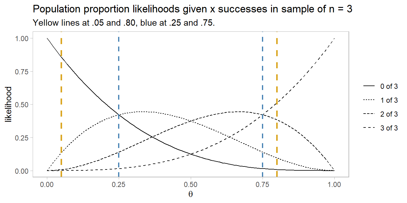
The blue lines demarcates the points where mixed results are as likely as unanimous results. A set of studies are likely to produce unanimous results only if the number of studies is fairly high \((\gt 1 - n / (n+1))\) or low \((< n / (n + 1))\).