1.1 Type I and II Errors

Either H0 or H1 is correct, and you must choose to either reject or not reject H0. That means there are four possible states at the end of your study. If your summary measure is extreme enough for you to declare a “positive” result and reject H0, you are either correct (true positive) or incorrect (false positive). False positives are called Type I errors. Alternatively, if your summary measure is not extreme enough for you to reject H0, you are either correct (true negative) or incorrect (false negative). False negatives are called Type II errors.

The probabilities of landing in these four states depend on your chosen significance level, \(\alpha\), and on the statistical power of the study, 1 - \(\beta\).

	H0 True	H1 True
Significance test is positive, so you reject H0.	False Positive Type I Error Probability = \(\alpha\)	True Positive Good Call! Probability = 1 - \(\beta\)
Significance test is negative, so you do not reject H0.	True Negative Good Call! Probability = (\(1 - \alpha\))	False Negative Type II Error Probability = \(\beta\)

\(\alpha\) is the expected rate of Type I errors due to summary measures that are extreme by chance alone. \(\beta\) is the expected rate of Type II errors due to summary measures that are not extreme by chance alone. In the IQ example, if the population mean was \(\mu\) = 100, any sample mean greater than qnorm(.95, 100, 15/sqrt(n)) = 104.5 would be mistakenly rejected at the \(\alpha\) = .05 significance level, a false positive. If the population mean was \(\mu\) = 106, any sample mean between 100 and 104.5 would be a mistakenly not rejected, a false negative.

What if the sample size had been n = 50 instead of 30? That would tighten the distribution curves of H0 and H1. Now if \(\mu\) = 100, a sample mean greater than qnorm(.95, 100, 15/sqrt(50)) = 103.5 would be mistakenly rejected (Type I error), and if \(\mu\) = 106, a sample mean between 100 and 103.5 would be a mistakenly not rejected (Type II error).

iq_range <- seq(90, 120, .01)
n2 <- 50

tmp <- data.frame(
  iq = iq_range,
  H0 = dnorm(iq_range, mean = mu_0,  sd = sigma / sqrt(n2)),
  H1 = dnorm(iq_range, mean = x_bar, sd = sigma / sqrt(n2))
)

alpha_x <- qnorm(.95, mu_0, sigma / sqrt(n2))
alpha_y <- dnorm(alpha_x, mean = mu_0, sd = sigma / sqrt(n2))

tmp %>% 
  pivot_longer(cols = c(H0, H1), values_to = "density") %>%
  mutate(alpha_beta = if_else((name == "H0" & iq >= alpha_x) | 
                                (name == "H1" & iq <= alpha_x & iq > mu_0), 
                              density, NA_real_)) %>%
  ggplot(aes(x = iq, color = name, fill = name)) +
  geom_line(aes(y = density), size = 1) +
  geom_area(aes(y = alpha_beta), alpha = .4, show.legend = FALSE) +
  geom_vline(xintercept = mu_0, linetype = 2, size = 1, color = "lightgoldenrod") +
  geom_vline(xintercept = x_bar, linetype = 2, size = .5, color = "steelblue") +
  geom_vline(xintercept = qnorm(.95, mu_0, sigma / sqrt(50)), 
             linetype = 2, size = .5, color = "gray80") +
  scale_color_manual(values = c("H0" = "lightgoldenrod", "H1" = "lightsteelblue")) +
  scale_fill_manual(values = c("H0" = "lightgoldenrod", "H1" = "lightsteelblue")) +
  annotate("text", x = x_bar - 4, y = .0075, label = "beta", parse = TRUE, 
           color = "steelblue") +
  annotate("text", x = x_bar - .5, y = .0075, label = "alpha", parse = TRUE, 
           color = "darkgoldenrod") +
  theme_light() +
  theme(panel.grid = element_blank(), legend.position = "top") +
  labs(
    title = glue("n = {n2} tightens the distributions."),
    fill = NULL, color = NULL, x = "IQ"
  ) +
  scale_x_continuous(breaks = c(90, 100, round(qnorm(.95, mu_0, sigma / sqrt(50)), 1), 105.6, 110, 120))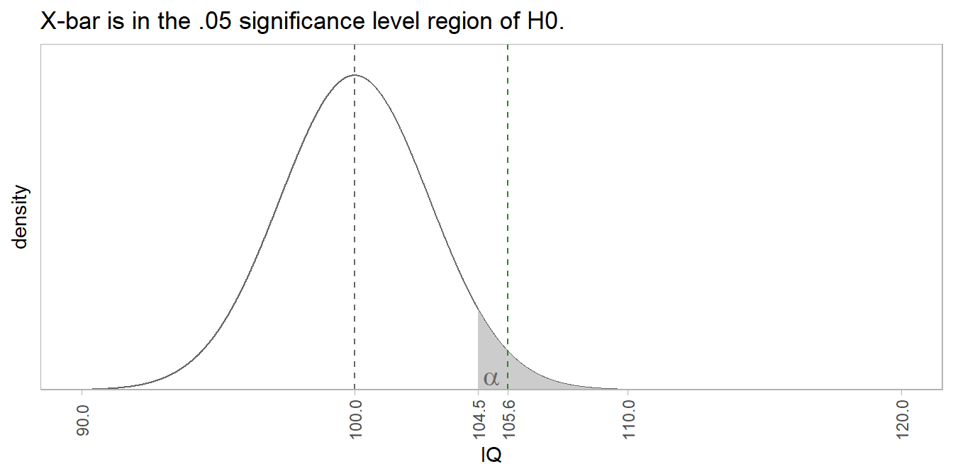

The ability to detect a difference when it exists (the true positive) is called the power of the test. Its measured by the area outside of \(\beta\). Changing n from 30 to 50 reduced the area in the \(\beta\) region, and therefore increased the power of the test.