0.2 Course Preparation
Your goals for this Getting Ready chapter are to:
- review the module study guide
- install R and RStudio software on your laptop/PC and carry out some simple test examples
- install Zotero
- read some overview articles on the role of data and Data Science in the 2020s
- complete the module questionnaire (which we will analyse using R in the Week 2 seminar)
- familiarise yourself with how to get help
i) Introducing the CS5702 Modern Data module
So what’s this module called ‘Modern Data’ all about? And why modern data? This is something we will go into more detail in Chapter 1 but as a sneak preview, these are unparalleled times when there is more data, and richer data available, than ever before. Coupled with more and more powerful analysis tools and generative AI, this affords us incredible opportunities to collect, clean, merge, analyse and visualise data both for good, and for less good purposes.
On a practical note, every module at Brunel has a unique code, in our case CS5702. The CS indicates it is owned and taught by the Department of Computer Science. Note also that all masters level modules are numbered 5nnn 5.
All the official information regarding this module (and indeed all modules at Brunel) can be found in their associated Study Guide. This is an important document, even if it seems a little bureaucratic, so please take time to review the contents. In it you will see two Learning Outcomes (LOs):
- “Appraise the quality of data and create tailored analysis plans for data preparation, data exploration and data management.” Underpinning this LO is the insight that data quality underpins any analysis. Problematic data will in all likelihood result in a misleading analysis and a waste of time and effort. So checking the data quality and any necessary cleaning is our starting point.
- “Critically evaluate and compare the strengths, the weaknesses and scope of statistical analysis methods for data exploration.” Here the LO reflects the fact that there is a seldom a single best way to undertake an analysis and in reality one makes judgements and tradeoffs. In fact the deeper you delve into Data Science and Statistics the more you will appreciate this!
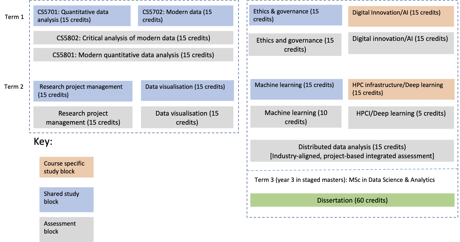
The Modern Data module shares two assessments with Quantitative Data Analysis (QDA) during Semester 1 as shown diagrammatically below. If you are studying full-time you will do an additional two modules one of which will depend upon whether you are enrolled for the MSc AI or MSc Data Science Analytics.
In addition, the Study Guide contains a week-by-week guide of topics. These correspond to the main chapters of this book. You will note that each week you have a one hour lecture and then on a broadly related topic a one hour seminar. The idea of the seminar is to be far more hands-on/interactive than the lecture. These are backed up by lab sessions which will principally run on a surgery-basis. However, you will need to spend additional time reading and trying out ideas working independently. This is a very practical topic and I strongly advocate exploration and experimentation.
ii) Install and test R and RStudio
This module, and other modules on your MSc, including CS5701 Quantitative Data Analysis, use R as a data analysis and statistical work horse. For a short overview and a discussion of the reasons for this choice, please see the section entitled “What is R and why do data scientists use it?” in Chapter 1. R is stable, free and available for most platforms, it has a wealth of features and is very widely used by statisticians, data analysts, scientists and machine learning researchers.
Therefore, you will first need to install R (Team 2022) and then RStudio (RStudio Team 2020). Note that the order is important.
Although in principle one could manage with just R, RStudio provides an easy way to manage not only R coding but the whole Data Science process. Ismay and Kim (2020) use the analogy of the difference between a car engine and the car dashboard. So we will use RStudio to ‘drive’ R, and not interact with it directly.

If you are feeling really impatient you can try some R code for yourself using an online R execution environment. Obviously it’s much better to install the software you need on your own computer, but as a simple expedient to get started, you can try this link to a free, web-based R editor. It will limit you to Base R. Another option is to create a (free) account with RStudio (posit) and use posit Cloud.
Installation steps
- Go to the Comprehensive R Archive Network that is universally known as CRAN6. Select the appropriate precompiled binary distribution for your computer (Mac/PC/Linux) to download R. It should be v4.0.0 or later.
- Go to RStudio’s website to download the RStudio IDE. Note that RStudio will not work unless you have previously installed R.
- Select the “RStudio Desktop FREE” option and click Download. NB you want the desktop, not the server version.
- Choose your operating system (Mac, Windows, or Linux).
- Select the ‘latest release’ on the page for your operating system (it should be 1.4 or later).
- Download and install the application.
- Launch RStudio.
Note that the icons for RStudio and R are superficially similar.

Make sure you launch the correct app. Generally you will want RStudio which is the righthand icon.
You will see that RStudio is split into panes. When you start you should see something like this. I recommend you check out my short (8mins) video introducing RStudio. Alternatively on YouTube, see this short introduction.
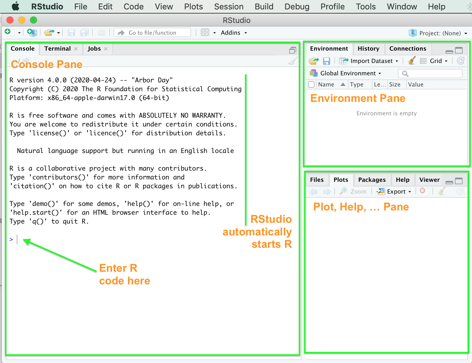
On the left is the Console Pane. Here you can type in your R code at the > prompt (highlighted by the green arrow ) followed by the Return key. It is mainly used for interactive tasks, e.g., interactively analysing some data or to test a command and see if it works. To the top right is the Environment Pane which shows the different variables and their values that you are using. Since RStudio has only just been launched and we haven’t done anything yet, this pane is empty. Likewise, the bottom right pane (where you can tab between Plots and Help, amongst other options) is also empty.
Now it’s time to run your first piece of R code which computes the answer to one plus one divided by 5. Change it so it computes two plus two multiplied by 5. NB The two lines starting with a hash symbol (#) are comments which are ignored by the R interpreter, however, they do help make your code easier to read for humans.
# Any line commencing with a hash is a comment, e.g., this one.
# R can evaluate arithmetic functions, the spaces are for aesthetic purposes only.
(1 + 1)/5
## [1] 0.4Let’s move on to a more complex and more useful R program. Don’t worry if you don’t follow all the details yet, as our main purpose is to get you used to RStudio and to begin to see the power of R.
In Computer Science a vector is one-dimensional array of the same data type. For example, we could have a vector of characters or integers. Each element is characterised by its position so we can have the first element, the second, the last and so forth. In R you can reference an individual vector element so v[1] <- 0 assigns zero to the first element of vector v just as v. We can also reference the vector in its entirety if we prefer.
The R program below generates two vectors of 1000 random numbers that both follow a normal distribution7. However, although they have the same standard deviation sd of 2, they differ in that they have slightly different means or centres of 10 and 11 respectively. The program then visually compares the two vectors r1 and r2 graphically by plotting the kernel densities. These are a kind of smoothed histogram: for a technical explanation see (Schucany 2004) and a rather nice visualisation from (Conlen 2020) 8.
# A simple R program to compare two vectors of random numbers

set.seed(42)     # set the random number generator seed so we get same output each time
nTrials <- 1000
m1 <- 10         # mean for random vector r1
m2 <- 11         # mean for random vector r2
sd <- 2          # standard deviation for the random numbers

# rnorm is a built in function. You can find out more by typing "?rnorm"
r1 <- rnorm(nTrials, m1, sd)   # Generate 1000 normally distributed numbers
r2 <- rnorm(nTrials, m2, sd)   # Generate 1000 numbers, with a different mean

plot(density(r1), main = "Kernel Density Plot: r1 and r2", col = "purple")
lines(density(r2), col = "red")   # Overlay density of r2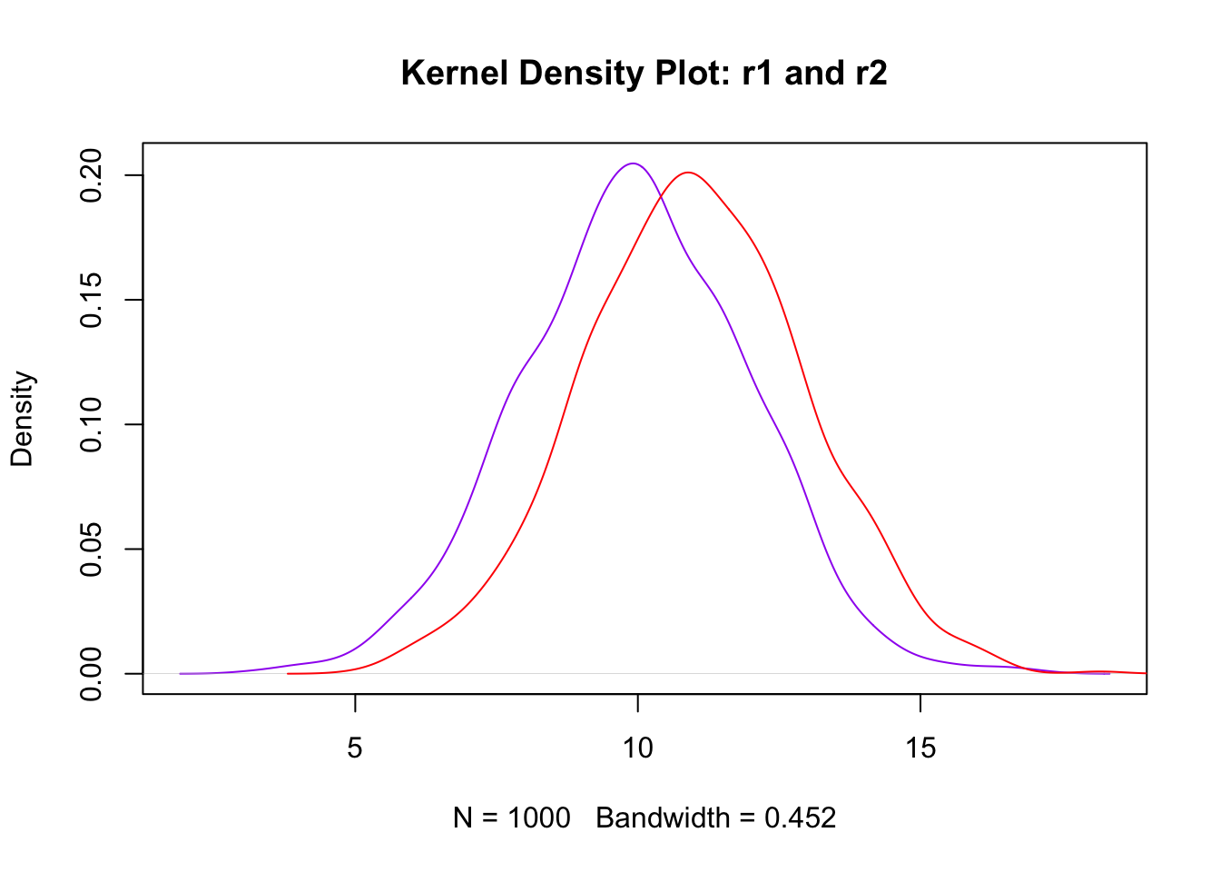
Looking at the R code, we see that the comments appear in green text. To some extent RStudio ‘understands’ R code and highlights different aspects of the syntax with different colours.
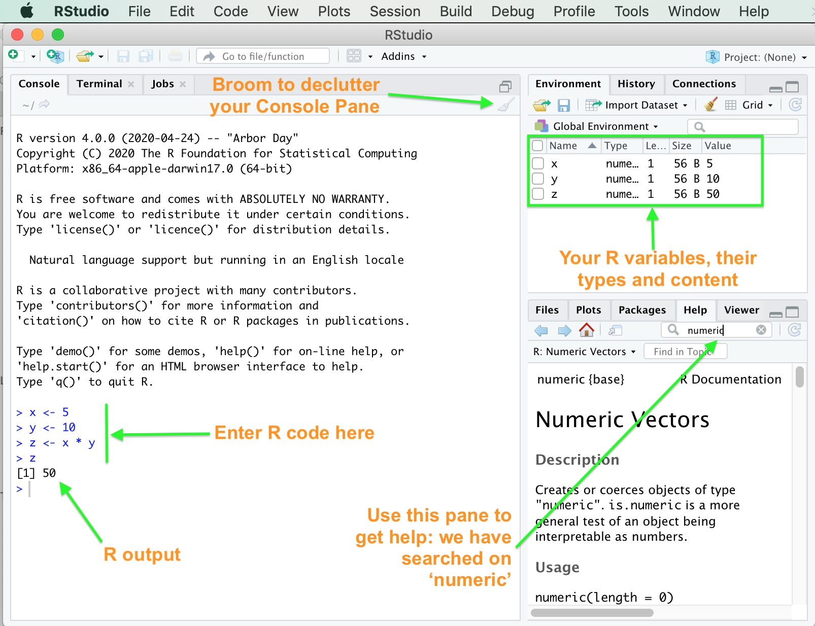
Below is the output of two superimposed density plots, a purple one for r1 and a red one for r2. I suggest you copy and paste the above program (use the icon in the top right corner when you mouseover the code) into the Console Pane of RStudio. When you execute it using the Return key note that the output will appear in the Plot Pane and the Environment Pane will be updated to reflect the contents of all the variables your program has created/manipulated (see the screenshot below ).
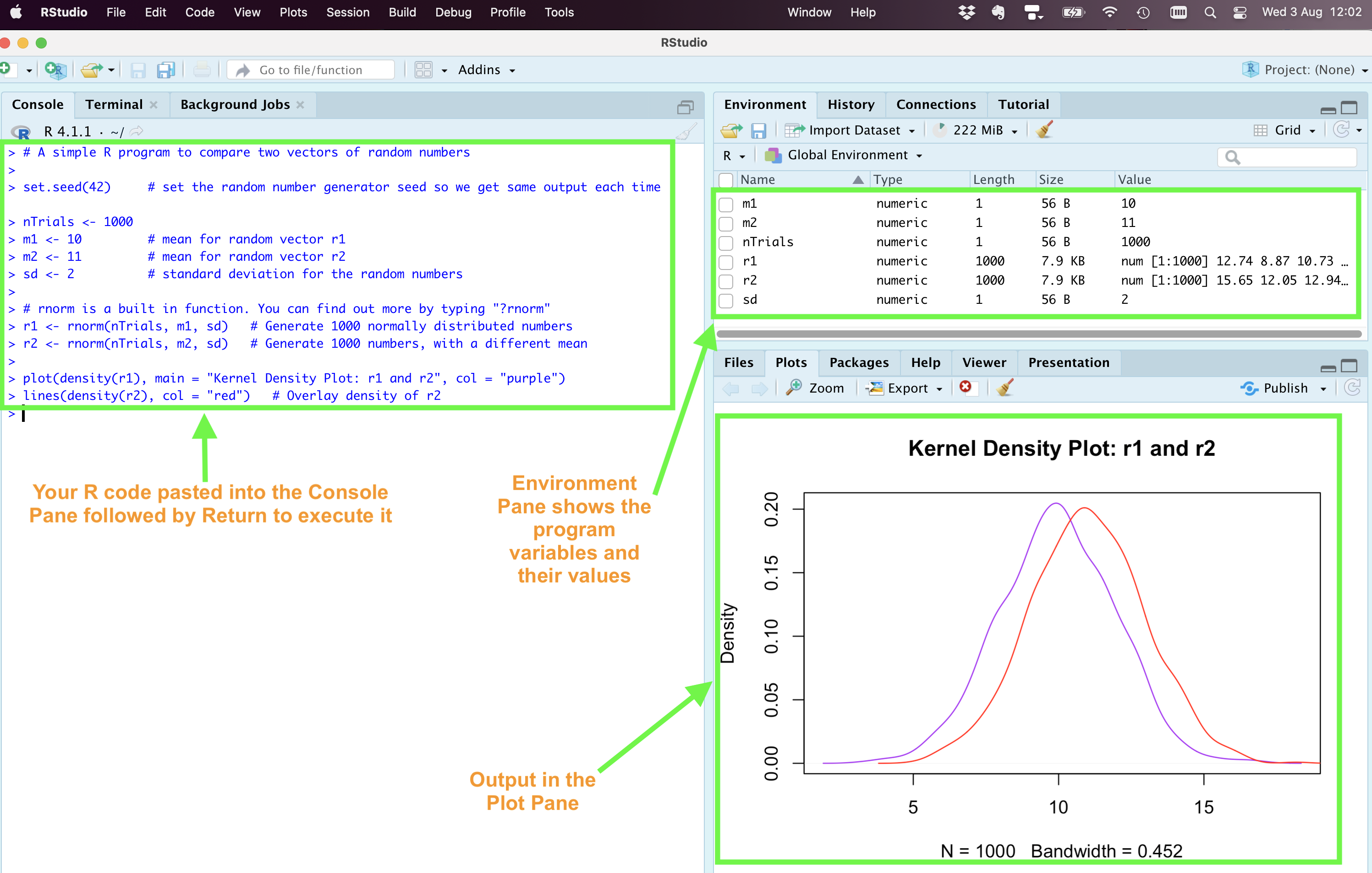
If you use any random number generator, e.g., rnorm() it’s a good idea to set the seed to some fixed value set.seed(nnn) where ‘nnn’ is some number chosen by you, so that if you re-run your code you will get the same output each time. This can really help testing and debugging. I have arbitrarily chosen 42 in set.seed(42) but it doesn’t matter.
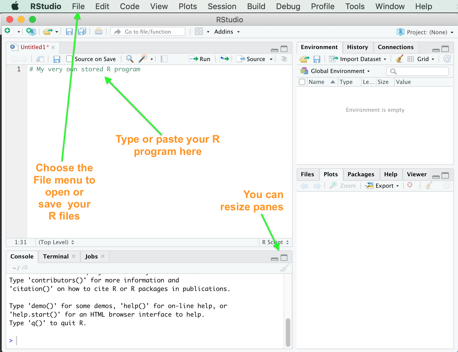
If you find typing/pasting R code into the Console Pane every time you want to execute it, is becoming tedious then you’re right! From the top menu bar choose File > New File > R Script and an empty pane will appear in the top right of the window named ‘Untitled1’ until you Save it as something. Note the file will be named <yourfilename>.R. You can get RStudio to save the file somewhere convenient by selecting the Session > Set Working Directory option. Now you execute the R, not by pressing Return as in the Console Pane, but by selecting the code you wish to execute and then clicking Run.
Once, you have successfully saved the R program you can start to experiment, e.g., try different standard deviations and means for the randomly generated data. You can also explore other ways of visualising the distributions, such as histograms and boxplots. Try hist(r1); hist(r2) and boxplot(r1, r2). NB slightly annoyingly, the hist() function will only take a single variable as an argument, whereas boxplot() will accept multiple arguments. Also note that ; is used when we are not using an end-of-line or carriage return to separate R commands.
When you Quit RStudio you will be prompted to “Save your workspace image”. I strongly advise you to select “Don’t Save” to prevent carry-over effects from one R session to the next. Under Preferences > General > Workspace you can set a Never save workspace option to prevent you having to answer every time you Quit RStudio.
Although initially RStudio might seem quite complicated, it’s an extremely useful and versatile Integrated Development Environment (IDE) for R. A lot more information can be found about RStudio:
- see this tutorial for more detail including loading and managing data (something we will cover in the next few weeks)
- the RStudio IDE cheatsheet
- blog from the RStudio team about the release of v1.4
- for an in depth information see the online book (Campbell 2020) available via the Brunel library
iii) Install Zotero
Reading is an important part of study and your time is precious, so use tools to make you as efficient and organised as possible. I highly recommend www.zotero.org however if you are already comfortable using an alternative , e.g., bibtex then stick with it. The crucial thing is to be systematic. You are also likely to find that Zotero will also be useful for the other modules you are studying and especially for your Individual Project.
Here is a link to a 7:50 min video on how and why you should install Zotero9.
iv) Some introductory data and data science reading
We are fortunate in that there is a vast range of books, tutorials, guides, blogs and other articles available in the general area of Data Science. However, to introduce you to the topic I suggest you read the following and try to answer the associated questions.
- What do we mean by data? It’s a term we use regularly but it’s hard to come up with a water tight definition. You might start with the Wikipedia article. Do you agree? Would you add anything?
- Next what do we mean by data scientist? Compare the webpage at Berkley with this webpage from prospects.ac.uk and the article entitled “what data-scientists really do according to 35 data-scientists” at the Harvard Business Review. Do they agree? Where do they differ? What do you think?
- Roger Peng has a thought provoking blog on “Tukey10, Design Thinking, and Better Questions”. But why should data scientists worry about questions? Surely this is up to the user? What do you think?
- Make sure you add these articles to Zotero and add your thoughts as attached notes.
v) Welcome to the module questionnaire
Please complete this short, anonymous questionnaire. This is completely optional, but if you do it this will help me (Martin Shepperd) better understand the range of backgrounds and expectations of this year’s cohort. It will also provide input to the Week 2 seminar. Even if you don’t answer the questions, please critically examine them.
This questionnaire has been created using Google Forms and the link is https://forms.gle/UPF46nDhnekd9qm16. Please try to complete questionnaire accurately to help us better understand the student cohort, but also try to step back and reflect on the questionnaire itself. What are the key design decisions? How could it be improved since very few things are perfect? We will discuss this in Week 1.
vi) Learn how to get help
This sub-section considers the problem of what to do if you get stuck? Suppose something doesn’t work? Sooner or later this is an experience we all face. Therefore this is important reading.
Fortunately there are a wealth of resources. It is unlikely that you will encounter a problem that hasn’t been previously encountered (and solved). So don’t despair! The following are some possibilities:
- find/read the relevant cheatsheet (RStudio maintains a large collection)
- perspiration e.g., see this five step approach
- talk it over with a fellow student
- Modern Data FAQs on the Brunel Blackboard VLE
- Stack overflow - be aware there is a protocol (basically good manners and respect). This includes checking whether somebody has already asked (and had answered) your question, and providing a minimal working example (MWE)
- Google which can work surprisingly well
- try an online R execution environment such as codingground but be aware this only supports core R (i.e., no extra packages). This can be really useful if you don’t have your laptop or your R installation is broken
- another option is the RStudio Cloud which allows you to run a virtual copy of RStudio over the web, however, you will need to set an account. The basic version is free.
- ask a member of the course team: in which case we require the following three things: (i) what output did you expect (ii) what actually happened and (iii) a minimal working example so the problem can be re-run. Thanks!
When seeking help, consider things from the perspective of the person you are asking. Suppose you say my “code doesn’t work” or “I’m stuck” or “I don’t understand”. How can they possibly help? So please provide THREE things: (i) the outcome you desire (ii) the outcome you actually get and (iii) a minimal working example (MWE) so that the problem can be reproduced.
References
Be aware that whilst most modules at Brunel contain both a study and an assessment component, in some instances these are separated as is the case for Modern Data, so CS5702 is a study block and it shares two assessment blocks (CS5801 and CS5802) with its ‘sibling’ study block CS5701 Quantitative Data Analysis.↩︎
CRAN is in actual fact a network of ftp and web servers around the world that mirror each other and have the latest versions of the code, packages and documentation for R.↩︎
In statistics a normal (or Gaussian) distribution is a type of continuous probability distribution for a real-valued random variable, which is characterised by being symmetric, having a single peak (mode) and having most observations cluster around the peak such that extreme values are very unlikely, but not impossible. Normal distributions have many useful properties and so are important in statistics.↩︎
As a technical aside the plots are quite basic in order to restrict the program to base R, e.g., no external packages in order to minimise complexity. Later, in the Chapter on Exploratory Data Analysis and Visualisation we will explore the {ggplot2} package which enables the production of highly flexible and sophisticated graphical output.↩︎
If you want some additional motivation, you can listen out for my neighbour’s mad dog barking towards the end of the recording!↩︎
John Tukey was a famous statistician who amongst other things pioneered the idea of exploratory data analysis (EDA).↩︎