5.3 Checking for quality
There is a definite ordering for any data quality process:
1. Identify problems …
2. then determine and document the response
- ignore (not recommended)
— clean
— impute
But first, let’s try to consider the different types of data quality issue that can arise.
5.3.1 Types of data quality issue
Validity: How closely the data meets defined business rules or constraints, e.g.,
Mandatory: Certain columns cannot be empty
Data-type: Values must be a certain data type
Range: Minimum and maximum values for numbers or dates
Uniqueness: A field or fields must be unique in a dataset
Set-membership constraint: Values must come from a set of discrete values/codes
Referential integrity: Constraints based upon multiple variables, e.g., marriage and age
Accuracy: How closely data conforms to a standard or a true value
Completeness: How thorough or comprehensive the data are
Consistency: Ensuring variables measured in the same way from different locations etc
Traceability: Being able to find (and access) the source of the data
Timeliness: How quickly and recently the data has been updated
Obviously this list is not exhaustive and there may well be additional domain specific criteria that must be taken into consideration.
5.3.2 Variance, a misunderstood and overlooked characteristic
There are two particular challenges:
- almost-zero-variance-features: these are problematic if all (or almost all) instances have the same value
- outliers: these are abnormal or unusual values
A particularly important topic is dealing with outliers.
Outliers are data items that lie an abnormal distance from other typical values in sample. Although various statisticians have offered more specific definitions, e.g., outside the whiskers of a boxplot it is generally a subjective and context dependent decision. For a more detailed overview see the NIST Handbook or for a more general review (Hodge and Austin 2004)
If an outlier is identified there are various possibilities, it could be:
- an error e.g., age = 155 years
- an interesting ‘edge’ case e.g., the most productive person in the sales team. (Grolemund and Wickham 2018) give an example of missing flight departure times as meaning the flight was cancelled so they add a new variable mutate(cancelled = is.na(dep_time).
5.3.3 Integrity checking
This can basically take two forms:
- with respect to the variable and its metadata, so for example, that value must be non-negative or within a particular range
- referential integrity where the checking is with respect to one or more other variables, for instance if a person is married they must be at least 16 (and in some countries, 18) years old. If this rule or constraint is violated then we know at least one value must be incorrect.
5.3.3.1 Using the R package validate
Data quality checking is such an everyday and necessary part of a data scientist’s work it will be no surprise that there are many useful packages to help. Of course, you can hand code everything from scratch, but there is no need and not necessarily much benefit.
One straightforward and useful package is {validate} 35. We show some simple features of this package with a hypothetical example based on some education data.
#  Load the {validate} package
library(validate)
# Load the example education data
fname <- "https://raw.githubusercontent.com/mjshepperd/CS5702-Data/master/CS5702_DatQualCheckingEg2.csv"
education.DF <- read.csv(fname, header = T, stringsAsFactors = T)
# Output the data frame in a nice formatted style
head(education.DF,nrow(education.DF))
## Education Sex Salary IncomeTax
## 1 BSc M 50000 15000
## 2 BSc M 45000 13500
## 3 BSc M 25000 7500
## 4 BSC F 0 0
## 5 BSc F 25000 7500
## 6 MSc F 55000 16500
## 7 MSc M 35000 90000
## 8 MSc F 90000 27000
## 9 PhD F 80000 24000
## 10 PhD M 145000 NAIn this Education example, we have a data frame with four variables or columns. The first two variables are factors (see the next section for more details on quality checking factors) and the remaining two are numeric (specifically integers).
Next, let’s look more carefully at the structure of the data frame.
## 'data.frame':    10 obs. of  4 variables:
##  $ Education: Factor w/ 4 levels "BSc","BSC","MSc",..: 1 1 1 2 1 3 3 3 4 4
##  $ Sex      : Factor w/ 3 levels "F","F ","M": 3 3 3 1 2 1 3 1 1 3
##  $ Salary   : int  50000 45000 25000 0 25000 55000 35000 90000 80000 145000
##  $ IncomeTax: int  15000 13500 7500 0 7500 16500 90000 27000 24000 NA
We can see some oddities like three levels for Sex. Using the table() function one check the counts/frequencies and the number of levels for Education and Sex.
##
##  F F   M
##  4  1  5
Having effective synonyms for the same factor level, i.e., F and F will cause potential problems and needs to be cleaned up.
It’s important to be systematic when undertaking quality checking. First, let’s define the quality checking rules many of which derive from, or are similar to, business rules. In this case let’s assume:
1. Education must “BSc”, “MSc” or “PhD” (this would be too restrictive in reality)
2. Sex must be “F” or “M” (actually this also might be restrictive, but for the purposes of this example)
3. Salary must be zero or more
4. IncomeTax must be zero or more
5. IncomeTax cannot exceed Salary
# Define the rules for {validate}
# Let's use the `validator()` to store the rules so they can be used more than once.
education.rules <- validator(okEduc = is.element(Education,c("BSc","MSc","PhD")),
                             okSex = is.element(Sex,c("F","M")),
                             NonNegSalary = Salary >= 0,
                             NonNegTax = IncomeTax >= 0,
                             TaxLessThanSalary = Salary >= IncomeTax)
Now we can apply these rules to our data set.
##                name items passes fails nNA error warning
## 1            okEduc    10      9     1   0 FALSE   FALSE
## 2             okSex    10      9     1   0 FALSE   FALSE
## 3      NonNegSalary    10     10     0   0 FALSE   FALSE
## 4         NonNegTax    10      9     0   1 FALSE   FALSE
## 5 TaxLessThanSalary    10      8     1   1 FALSE   FALSE
##                                      expression
## 1 is.element(Education, c("BSc", "MSc", "PhD"))
## 2                  is.element(Sex, c("F", "M"))
## 3                          Salary - 0 >= -1e-08
## 4                       IncomeTax - 0 >= -1e-08
## 5                  Salary - IncomeTax >= -1e-08
We can also check this graphically, e.g., with a bar chart.
## Warning: The 'barplot' method for confrontation objects is deprecated. Use
## 'plot' instead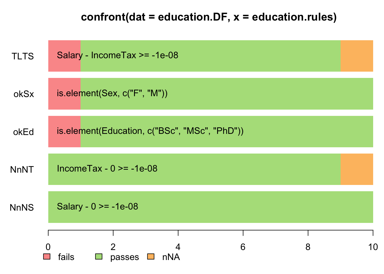
This reveals that there is a problem with IncomeTax since one value is missing, i.e., equal to NA and therefore this causes a problem with the quality rule that Salary >= IncomeTax and a second instance where Salary is actually less than IncomeTax (row 7).
To more systematically determine where a quality check is violated you can use the aggregate() function from {validate}.
##    npass nfail nNA rel.pass rel.fail rel.NA
## 1      5     0   0      1.0      0.0    0.0
## 2      5     0   0      1.0      0.0    0.0
## 3      5     0   0      1.0      0.0    0.0
## 4      4     1   0      0.8      0.2    0.0
## 5      4     1   0      0.8      0.2    0.0
## 6      5     0   0      1.0      0.0    0.0
## 7      4     1   0      0.8      0.2    0.0
## 8      5     0   0      1.0      0.0    0.0
## 9      5     0   0      1.0      0.0    0.0
## 10     3     0   2      0.6      0.0    0.4
This is of course just scratching the surface but hopefully it provides a feel for what can be done using R to check the quality of a data set.
5.3.3.2 Problems with factors
Factors are a special, and very useful, type of character string in R. They are characterised by a relatively few levels (i.e., distinct values) \(k\) such that \(k \ll n\), where \(n\) is the number of observations or cases. A good example is ethnicity; a bad example is email address which is likely to be unique to each observation. Factors often form the basis for data analysis questions e.g., are there any differences between ethnicities?
Depending upon the data input mechanism synonyms, differences in case, trailing and leading spaces can lead to R identifying spurious levels that will interfere with our analysis. For example,
- ‘Y’ or ‘y’ or ‘Yes’ or ‘T’ etc
- Trailing or leading spaces e.g., ’ Y’, ‘Y’ or ‘Y’
Consider the following very simple example based on the factor gender which might be important to investigate questions in our exploratory data analysis.
# Suppose we wish to check the quality of previously defined factor gender.
# Use the table function to check for levels
table(gender)
## gender
## F F m M
## 7 2 1 9A useful function to get counts by level for a factor is table(). In the above example we see that there are actually four levels rather than the two we intended indicating three observations with synonyms (i.e., “F” and “m”).
Jumping ahead we can fix these problems with a conditional assignment.
# Replace observations containing "m" with "M"
gender[gender == "m"] <- "M"
# Check the new frequencies by level
table(gender)
## gender
## F F m M
## 7 2 0 10Using table() we now see we have ‘lost’ the lower case level since the frequency is now zero, although R still ‘remembers’ the existence of this level.
Extend the cleaning of the factor gender to deal with the “F” level by removing the trailing space. Check that you have been successful by seeing that the “F” count has increased from 7 to 9.
References
The {validate} package is described with some useful vignettes by Mark P.J. van der Loo in The Data Validation Cookbook↩︎