4.3 Spatial stratified sampling with QGIS

If we look at the following map, we can see that the city has areas with more built up land than others.

The most suitable stratification in this case, where we have no knowledge about neighborhoods in the city or other significant characteristics of the city would be to use a spatial characteristic and divide La Plata into strata by land use and land cover. Therefore we will create strata according to built up and non built up areas based on satellite imagery provided by the Copernicus Land Monitoring Service global maps of land cover & cover changes and related surface area statistics in QGIS.

4.3.1 Land use change raster

To download the land use raster go to the following link - https://lcviewer.vito.be/2015 and select the download option to choose the area of analysis. (See 4.17)

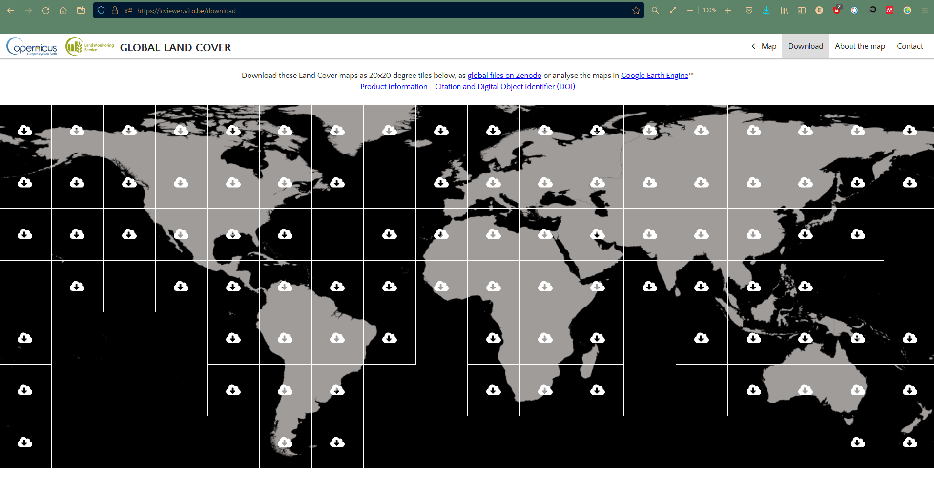
Figure 4.17: Land Use Map by Copernicus Land Monitoring Service

Next, we will upload the land use and land cover raster layer to QGIS, similar to the steps in 3.1. (See 4.18)

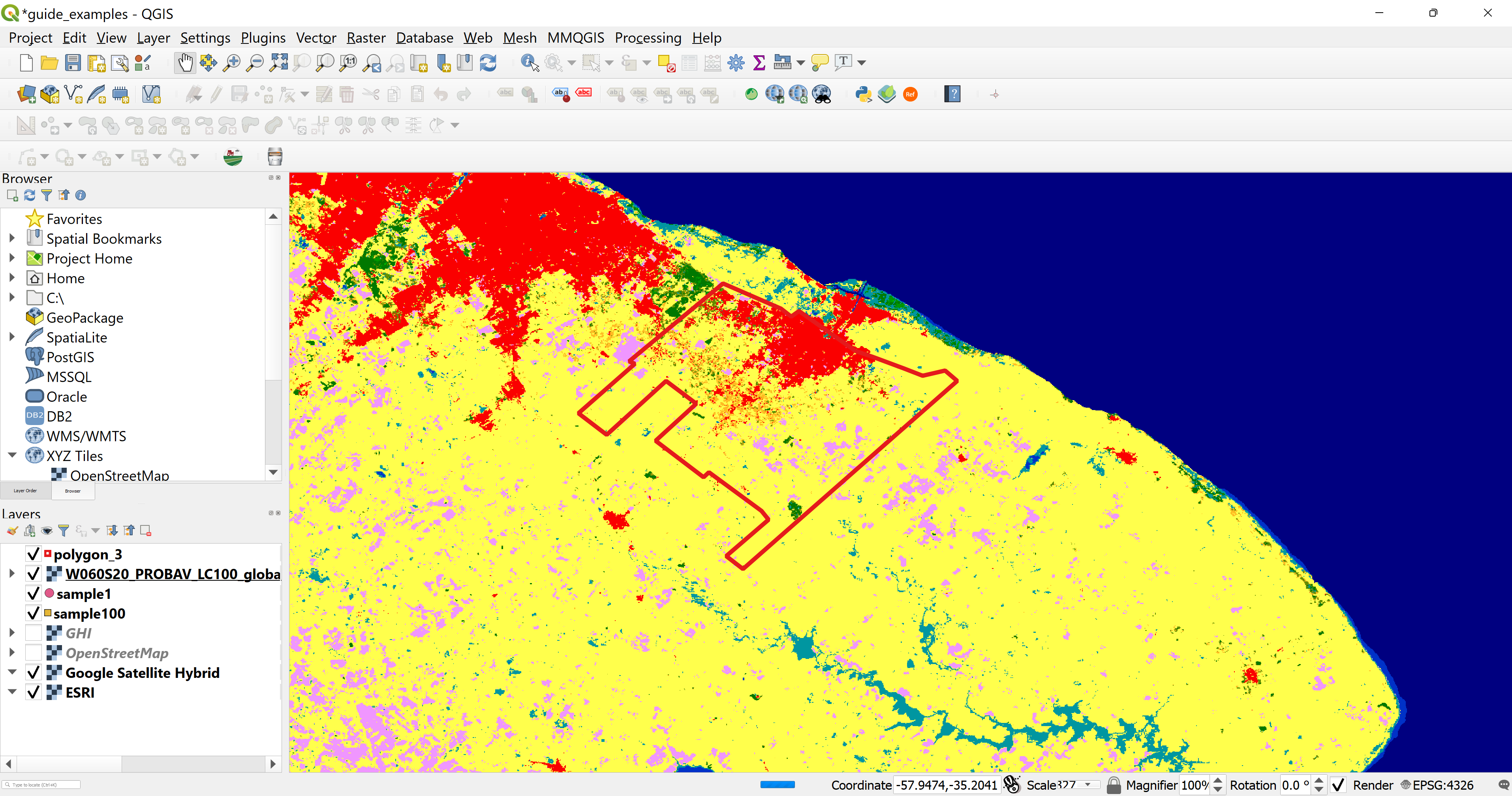
Figure 4.18: La Plata Land Use and Land Cover in QGIS

Then we would like to keep only the part of the raster that falls under the administrative border of La Plata. This can be done by going to Raster menu, selecting the Extraction option, and clicking on Clip Raster by Mask Layer…. (See 4.19)

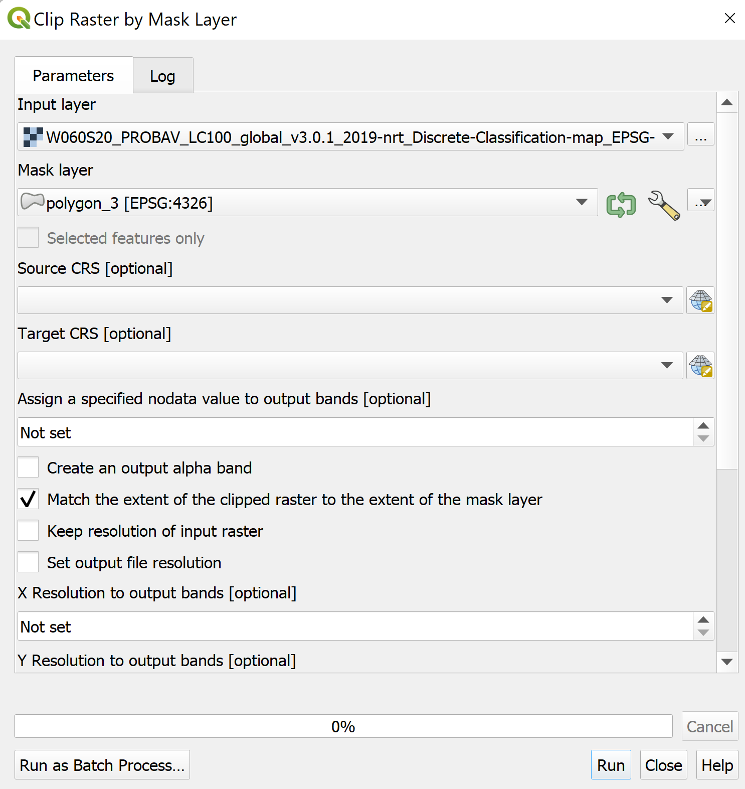
Figure 4.19: Clip Raster by Mask Layer Dialog

The dialog window will open, in it we can enter our Input layer the raster to be clipped, the Mask layer which is polygon_3, and save the new raster as laplata_landuse. (See 4.20)

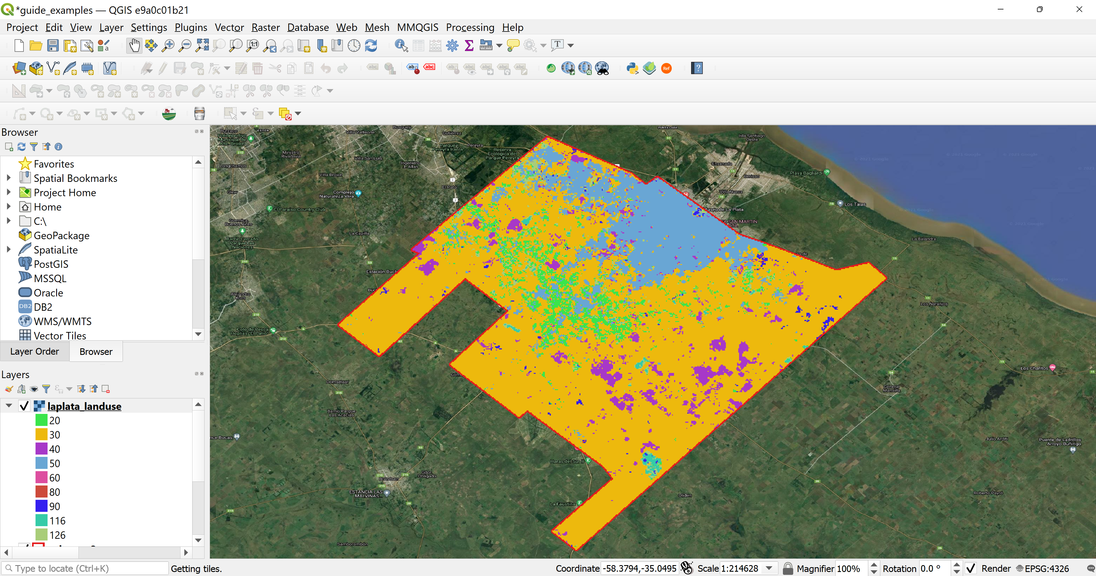
Figure 4.20: Clip Raster by Mask Layer Output

According to the Copernicus Land Monitoring Service global maps of land cover & cover changes and related surface area statistics web browser, the pixel values that are between 50-60 are defined as built up area. We will reclassify the raster image so the pixels between 50-60 will be given the value 1 and all the other pixels 0.

In the Processing Toolbox search bar we can search for the tool we would like to use - Reclassify by table. Then the algorithm configuration window will open and we can choose our raster layer laplata_landuse and the click on the Reclassification table parameter. (See 4.21)

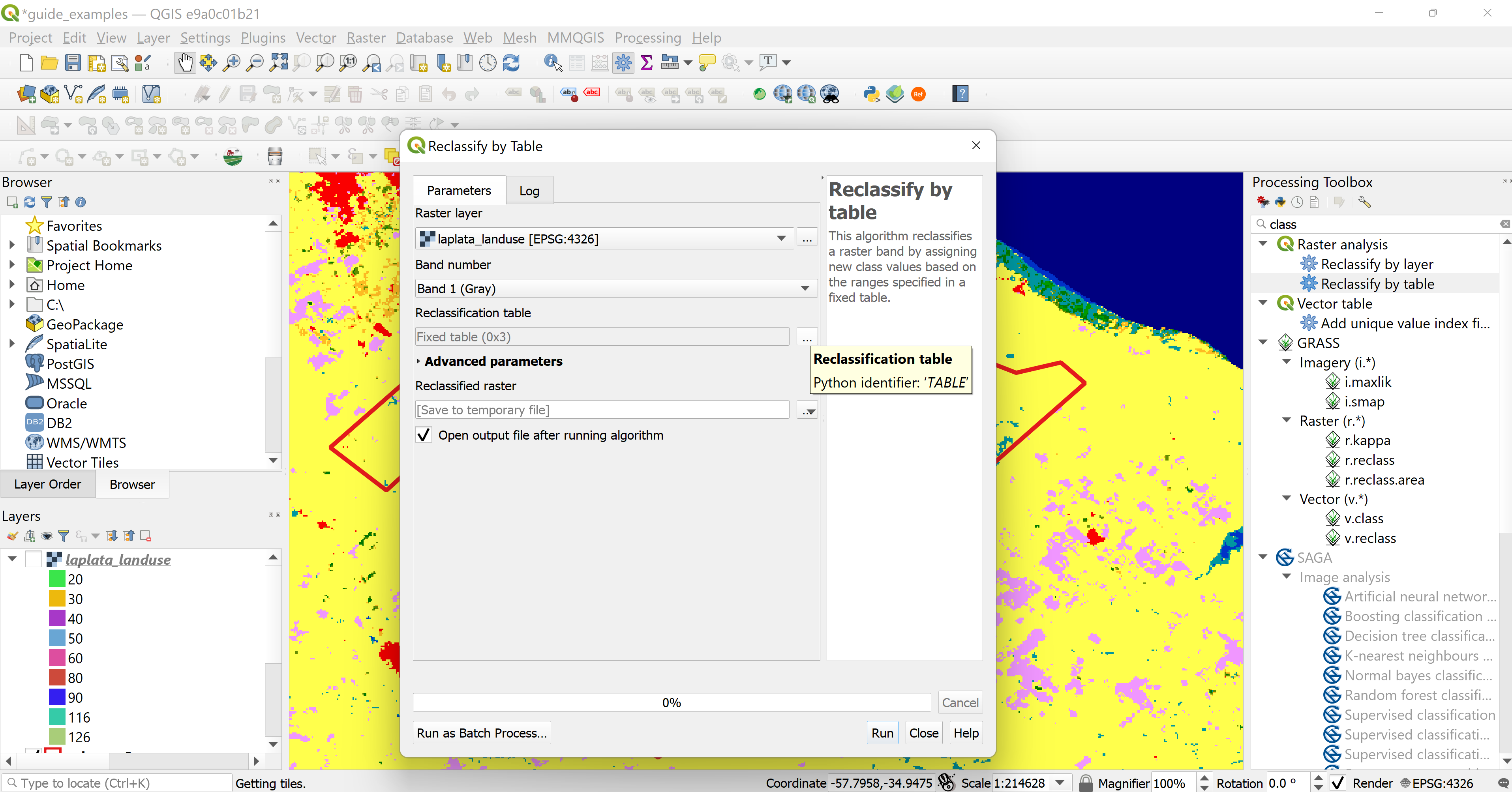
Figure 4.21: Reclassify by Table

In the Reclassification table we will set the values as seen in figure 4.22 and after we press OK we check the Advanced parameters and make sure that the Range boundaries are correct. (See 4.23)

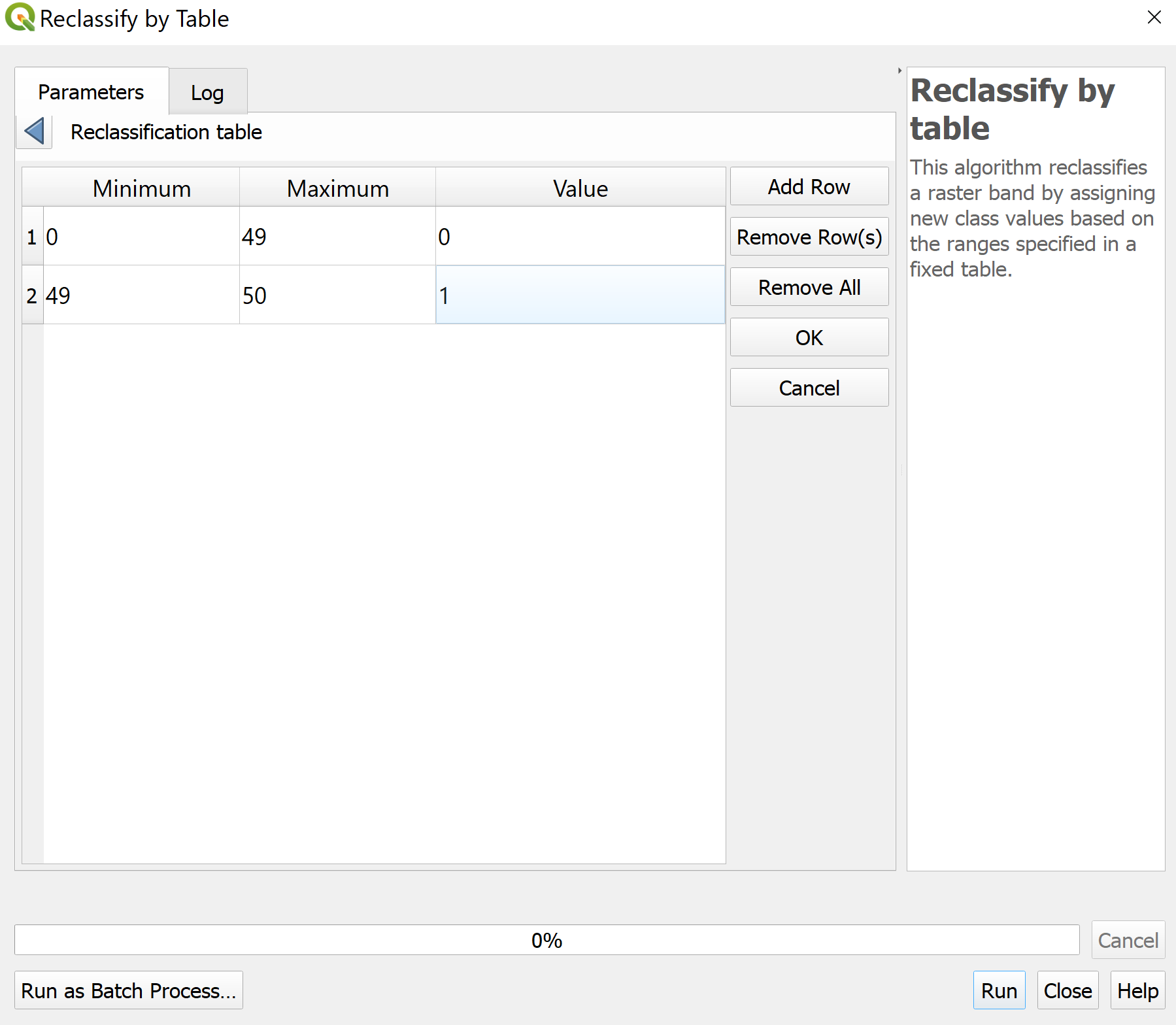
Figure 4.22: Reclassification Table

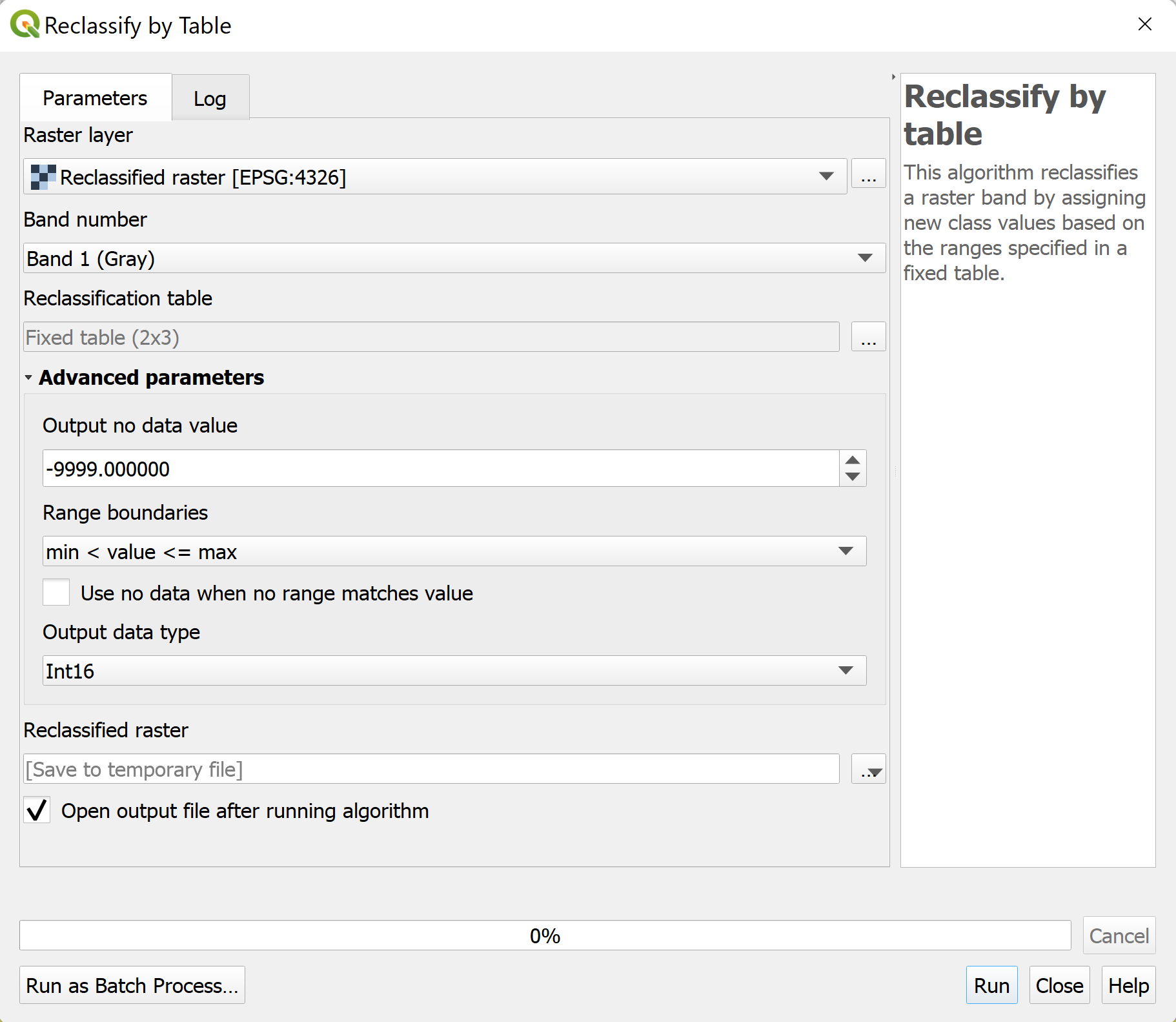
Figure 4.23: Advanced Parameters

As a final step we will go to the Symbology of the laplata_landuse layer and change the Max value to 1. Then we can see clearly which part of the city is built up and which is not. (See 4.24)

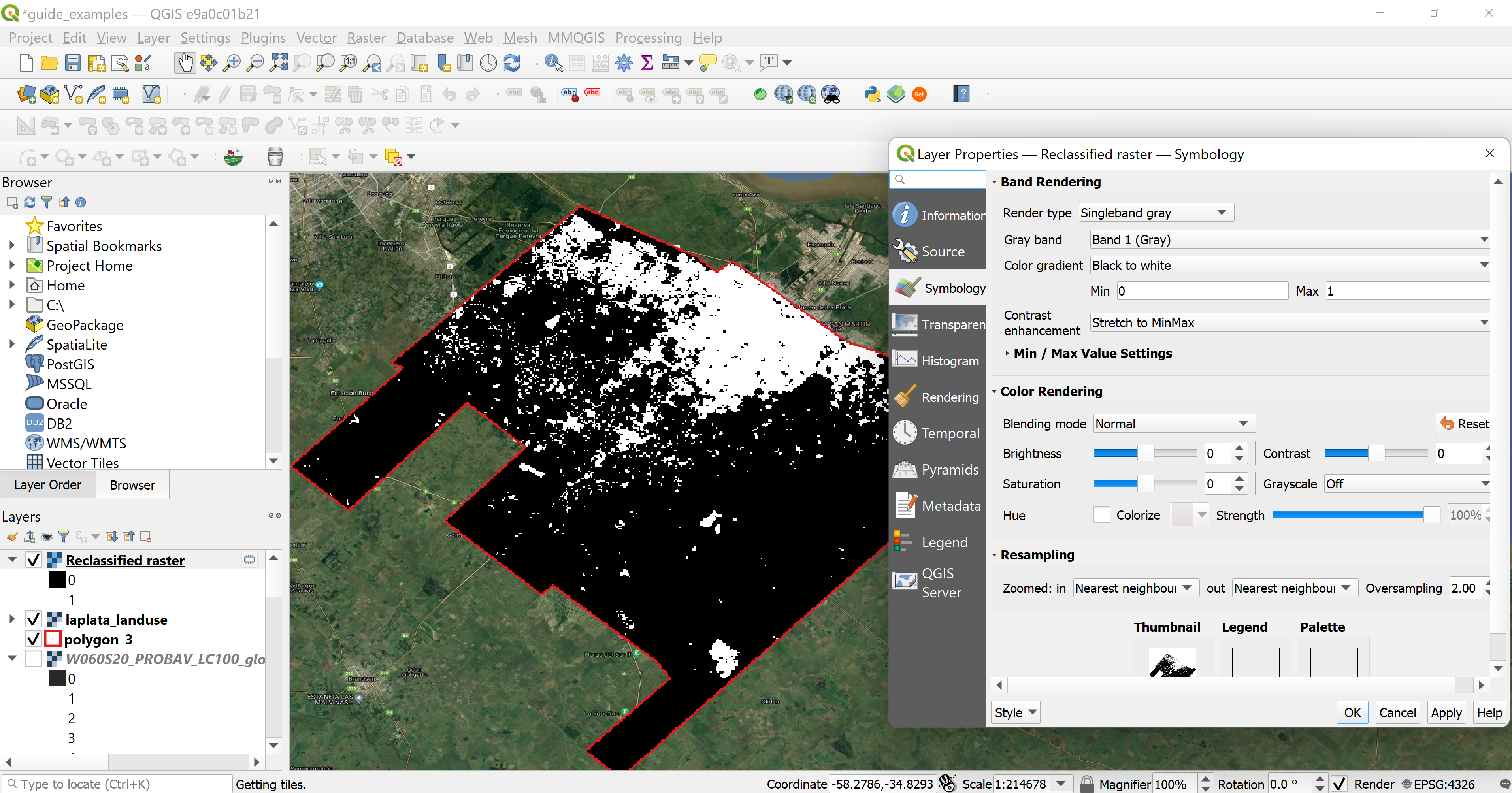
Figure 4.24: La Plata - Built Up and Non Built Up Area Classification

4.3.2 Raster to polygons

To compute spatial random points for each strata, we need to convert the reclassified raster to two vector layers - one for the built up area and another for the non built up area. For this process, we will use the Raster Conversion algorithm Polygonize (Raster to Vector)…. (See 4.25)

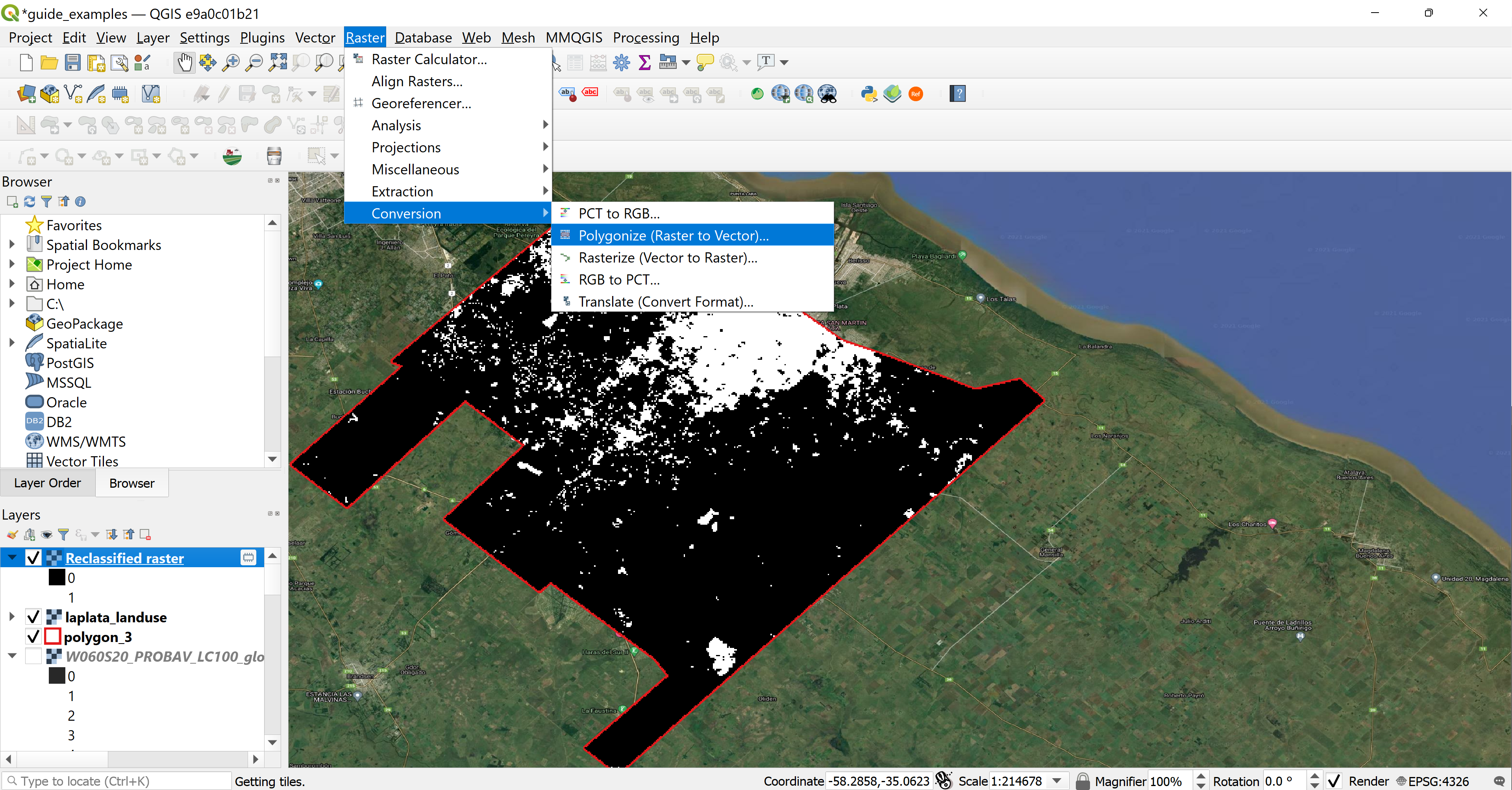
Figure 4.25: Polygonize (Raster to Vector)

The Polygonize (Raster to Vector)… window dialog will open and we will put the Reclassified raster layer as the input layer. (See 4.26)
The out put can be seen in figure 4.27.

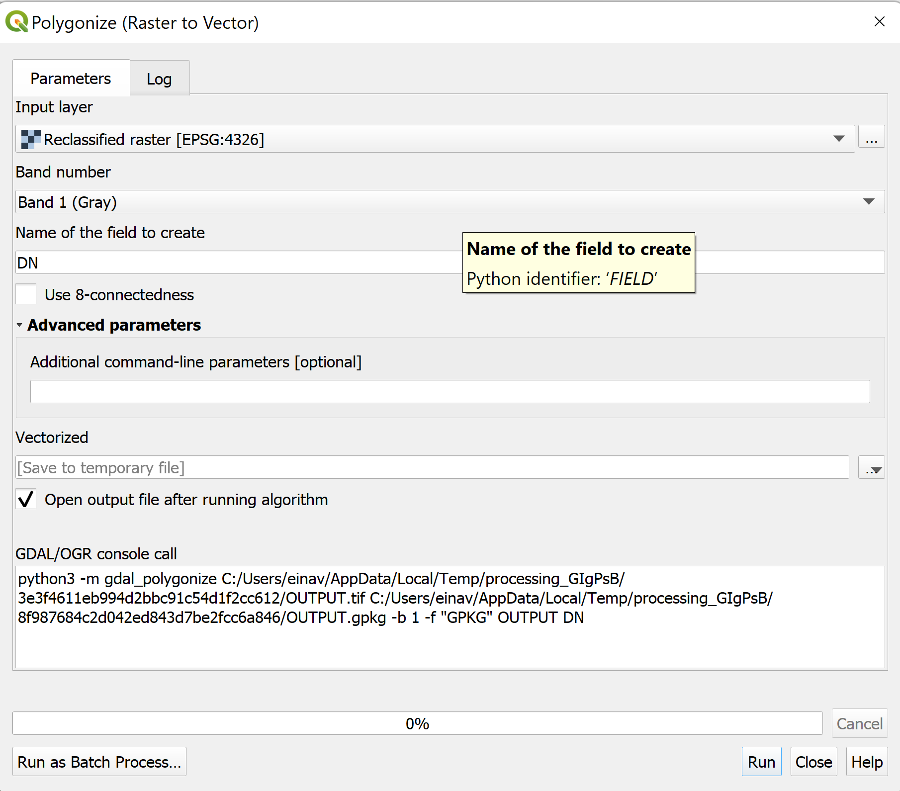
Figure 4.26: Polygonize (Raster to Vector) Dialog

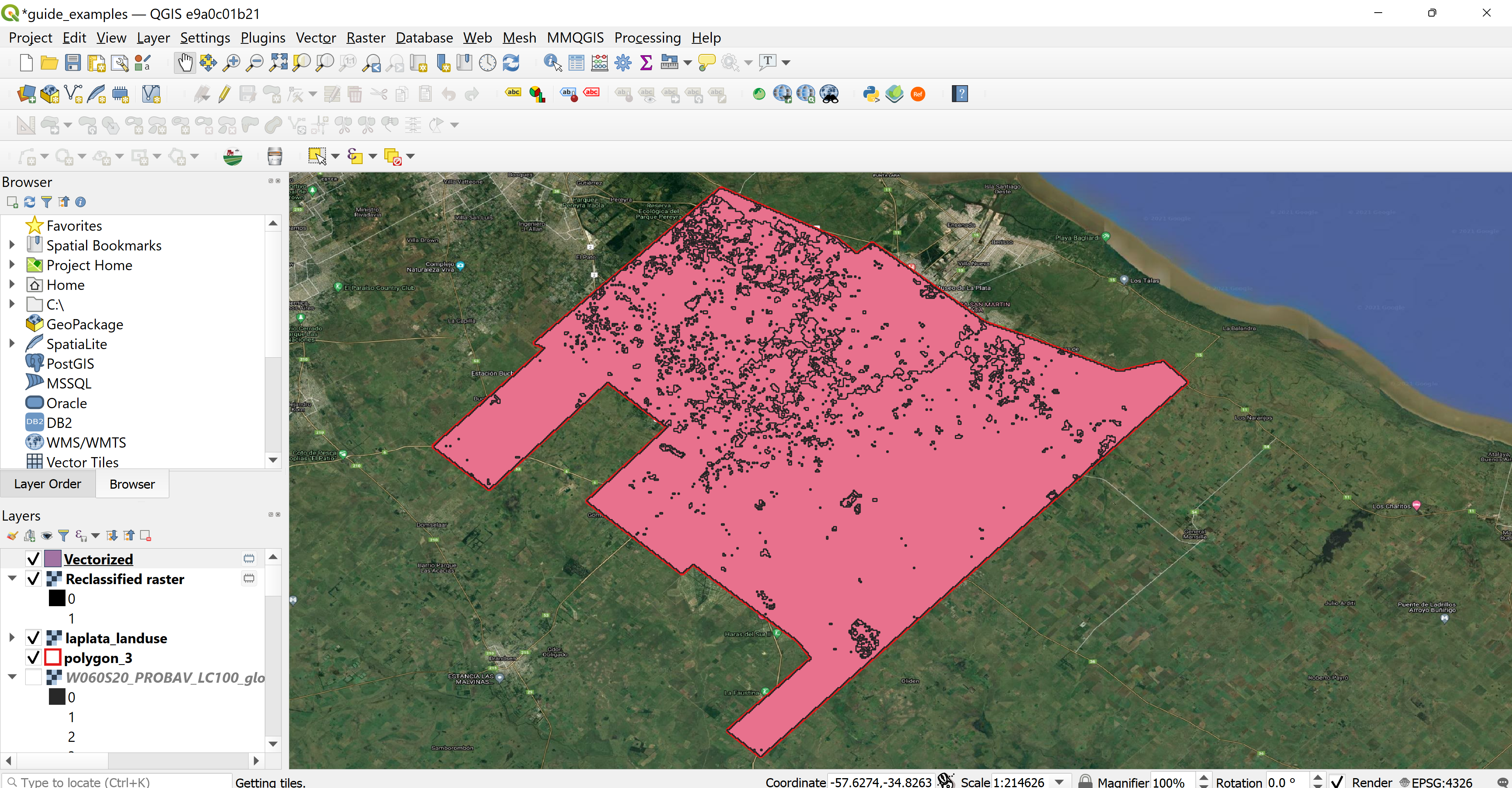
Figure 4.27: Polygonize (Raster to Vector) Output

Next, we will open the Vectorized layer’s attribute table and click on the Select features using an expression… option. (See 4.28) When the dialog window will open we will create an expression to first select all the DN values that belong to the non built up area. (See 4.29) Then we can right click on the Vectorized layer, select Export, Save Selected Features As… and save the non built up area as a vector layer in our directory. (See 4.30)

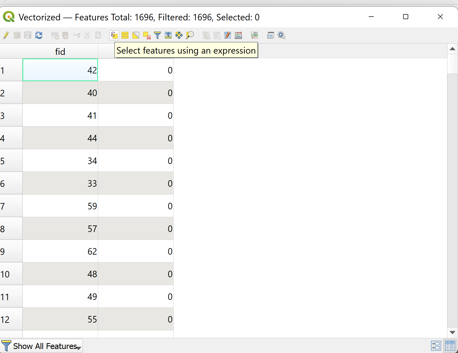
Figure 4.28: Vectorized Layer Attribute Table

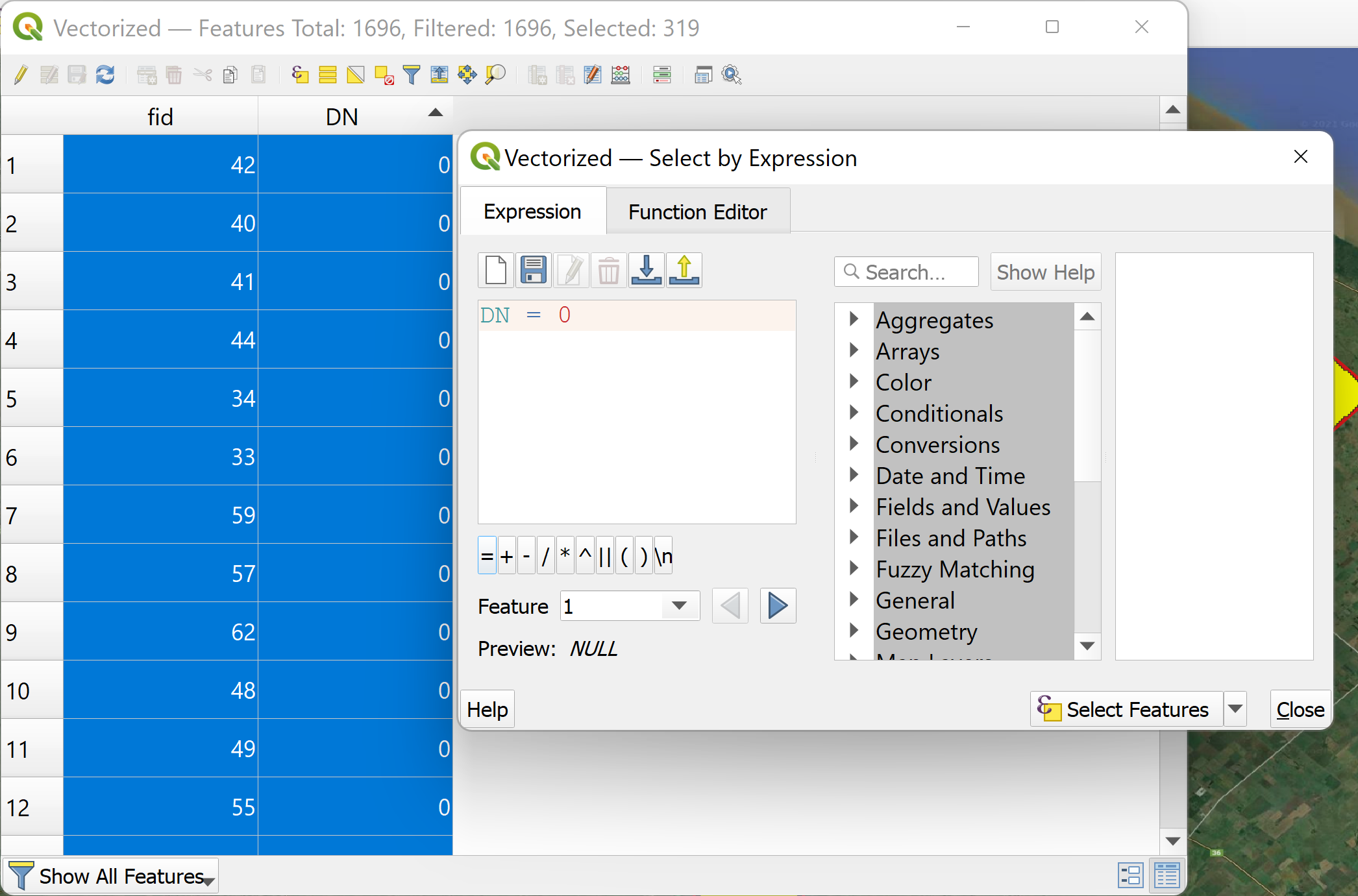
Figure 4.29: Select Features Using An Expression

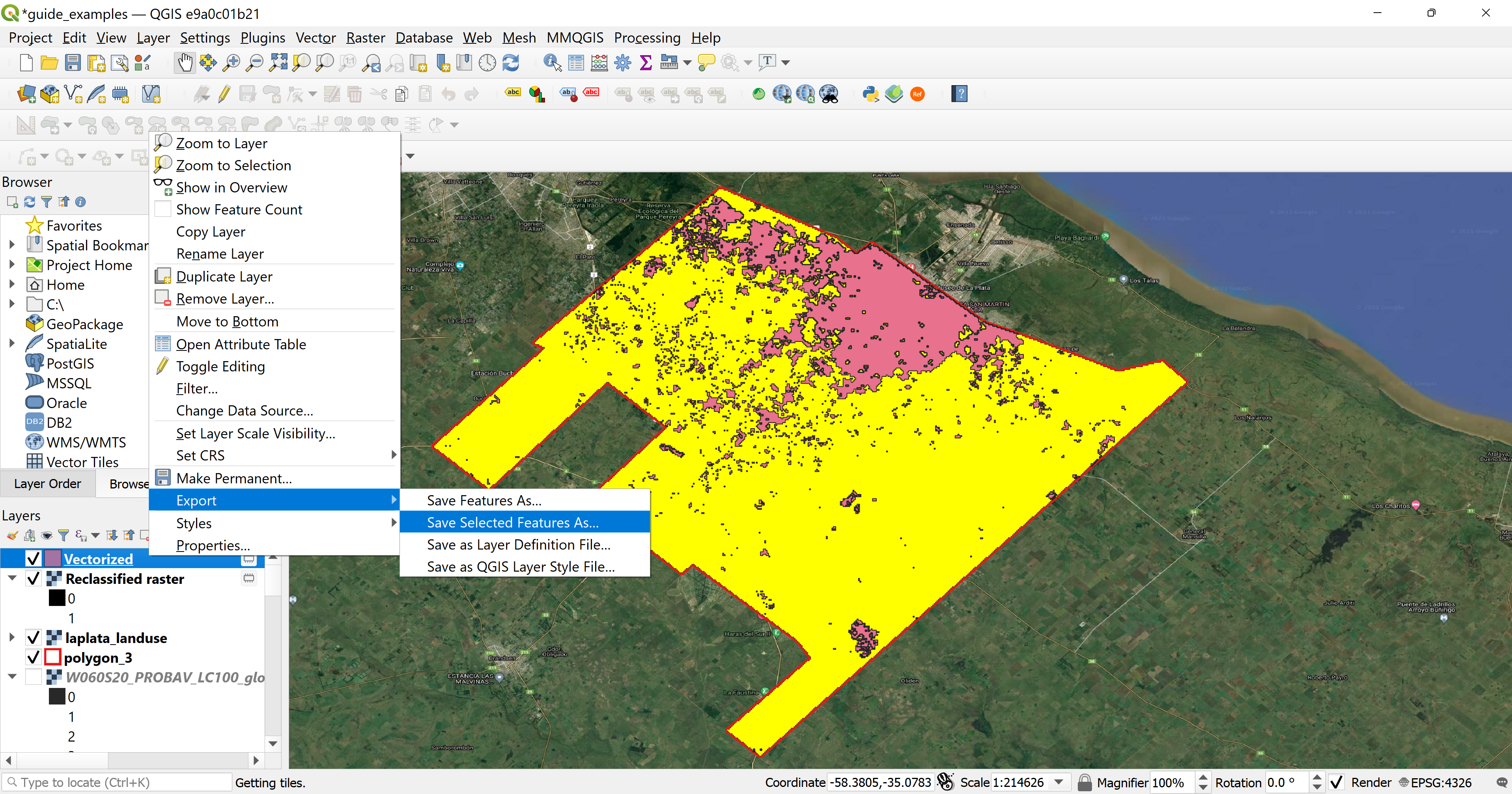
Figure 4.30: Select Features Using An Expression

Then repeat the process for the built up area. The result vector layers can be seen in figure 4.31 with the purple layer indicating the non built up area and the pink the built up area.

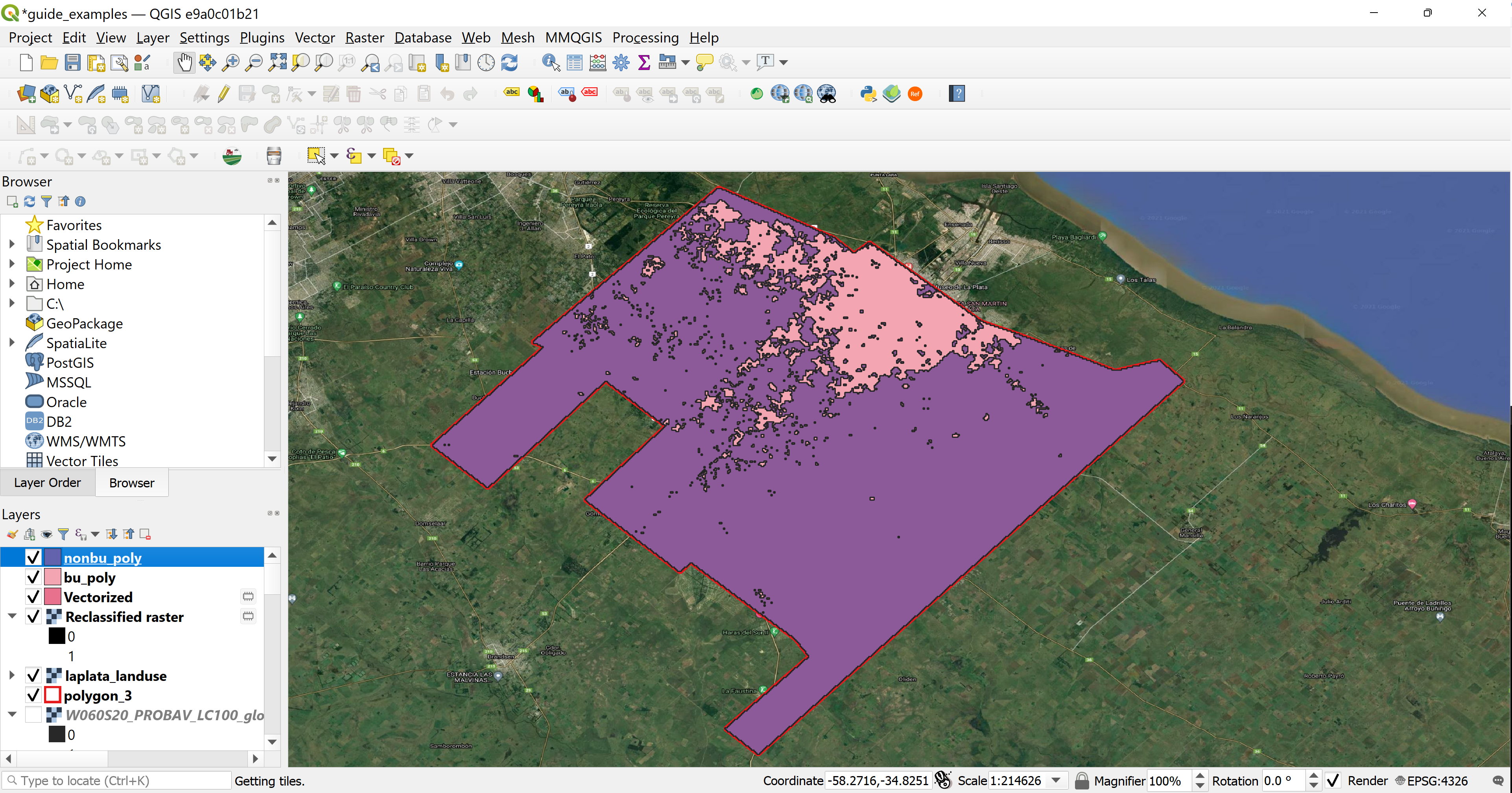
Figure 4.31: Built Up and Non Built Up area Vector Layers

Now that we have two strata, we will once again compute spatial random points as described in section 4.2, and then digitize them according to sections 4.2.2 and 4.2.3.