4.2 Spatial random sampling with QGIS

To create a spatial random sample in QGIS we will need the city’s administrative borders polygon. (See 4.1)

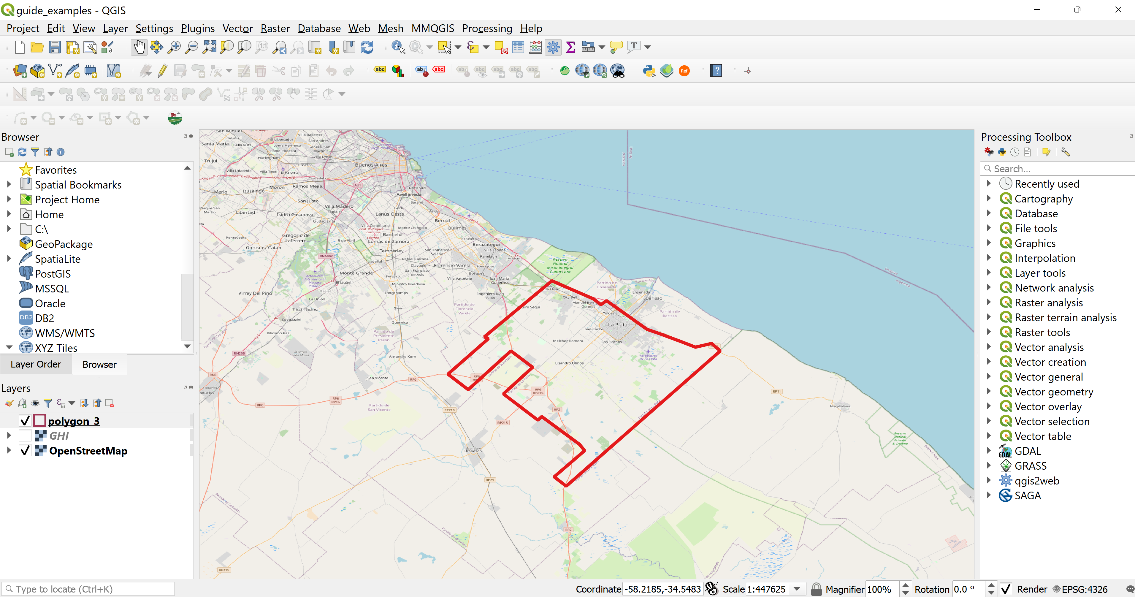
Figure 4.1: La Plata Administrative Border

Next, we will go to the Vector Menu, select the Research Tools option and click on the Random Points in Layer Bounds. This algorithm creates a new point layer with a given number of random points, all of them within the extent of a given layer. (See 4.2)

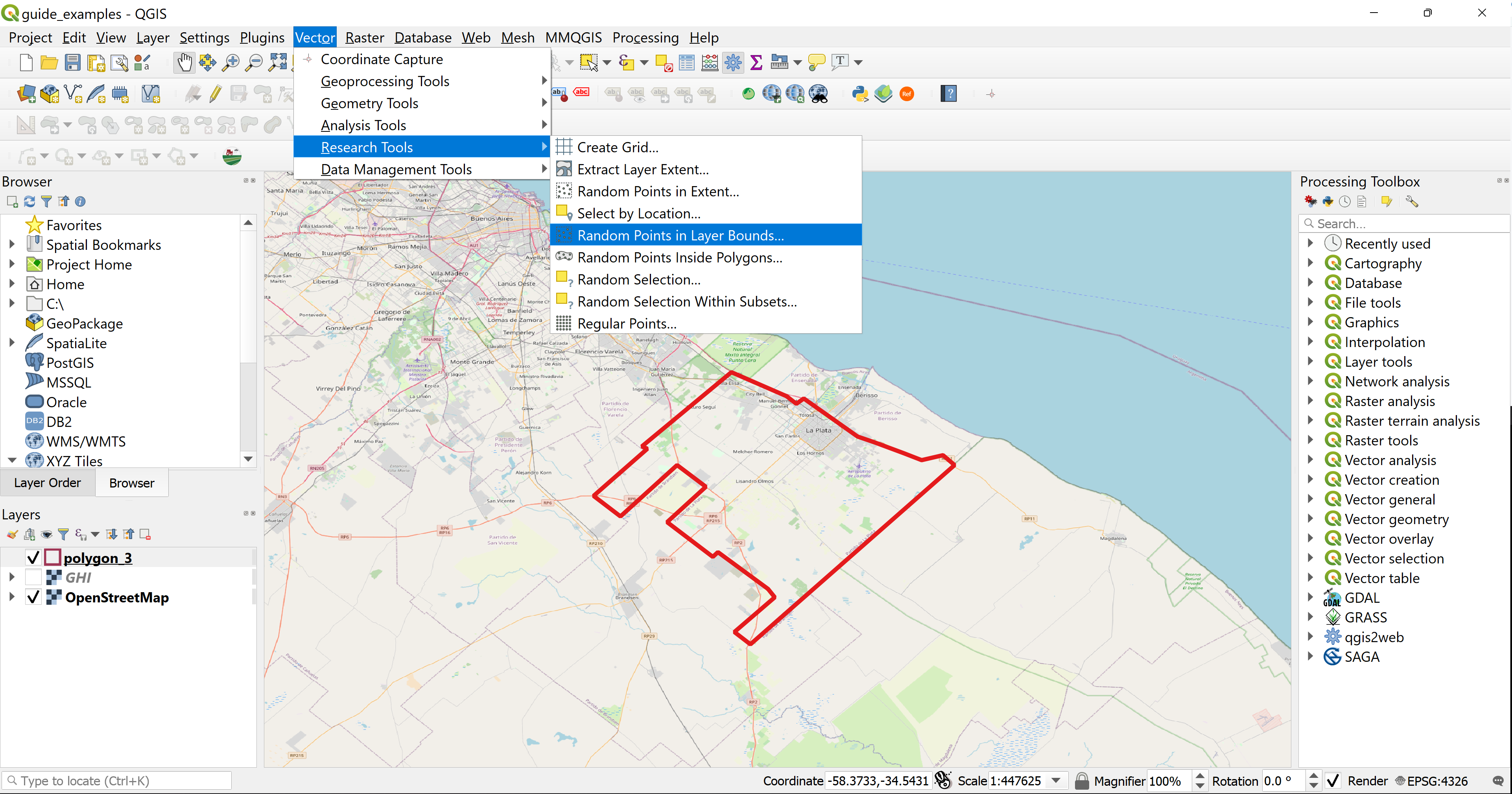
Figure 4.2: Random Points in Layer Bounds

The algorithm dialog window opens and we will fill in the parameters according to our analysis. The input layer of the administrative borders of La Plata is called polygon_3, first we will create 100 random points in the layers extent and save the file as a shapefile by the name sample1. (See 4.3)

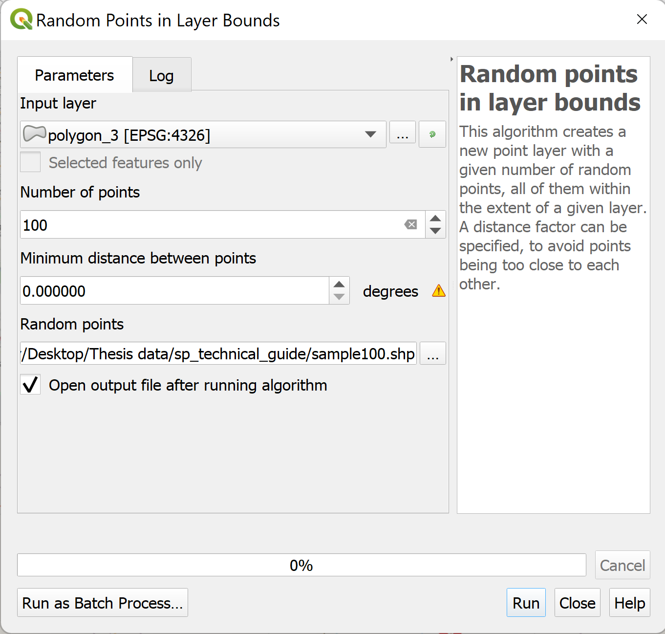
Figure 4.3: Random Points in Layer Bounds Dialog

We can see that the layer sample1 is uploaded to our QGIS interface. (See 4.4)

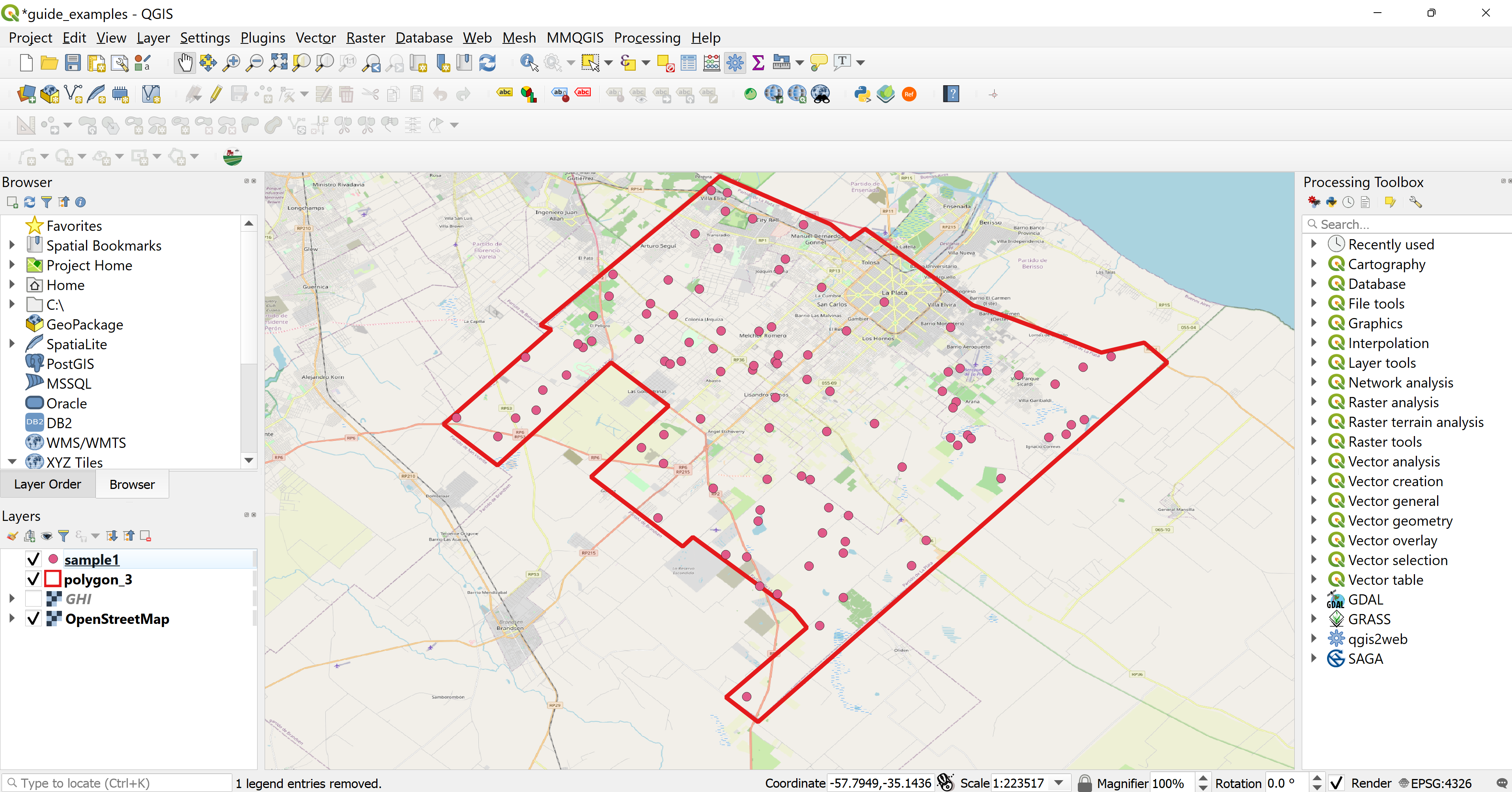
Figure 4.4: Random Points in Layer Bounds Output Layer in QGIS

4.2.1 The QMS plugin

Now that we created 100 sample points in the administrative borders of La Plata, we need to see where does the point fall. To do so, we will use QMS to add a TMS layer to the QGIS interface. There are many different TMS that are available in QMS (here), the ideal layer would be the one with a high resolution that was updated recently.
In this project, we will use two TMS layers to compare and achieve the best accuracy while digitizing the building rooftops.

To add the QMS plugin to QGIS, click on the Plugins menu and select the Manage and Install Plugins… option. (See 4.5)
The Plugins Dialog will open, there we can see all the plugins installed in our QGIS, in the search bar we will type QMS and see if the plugin needs to be installed or already exists in the plugin library. (See 4.6)

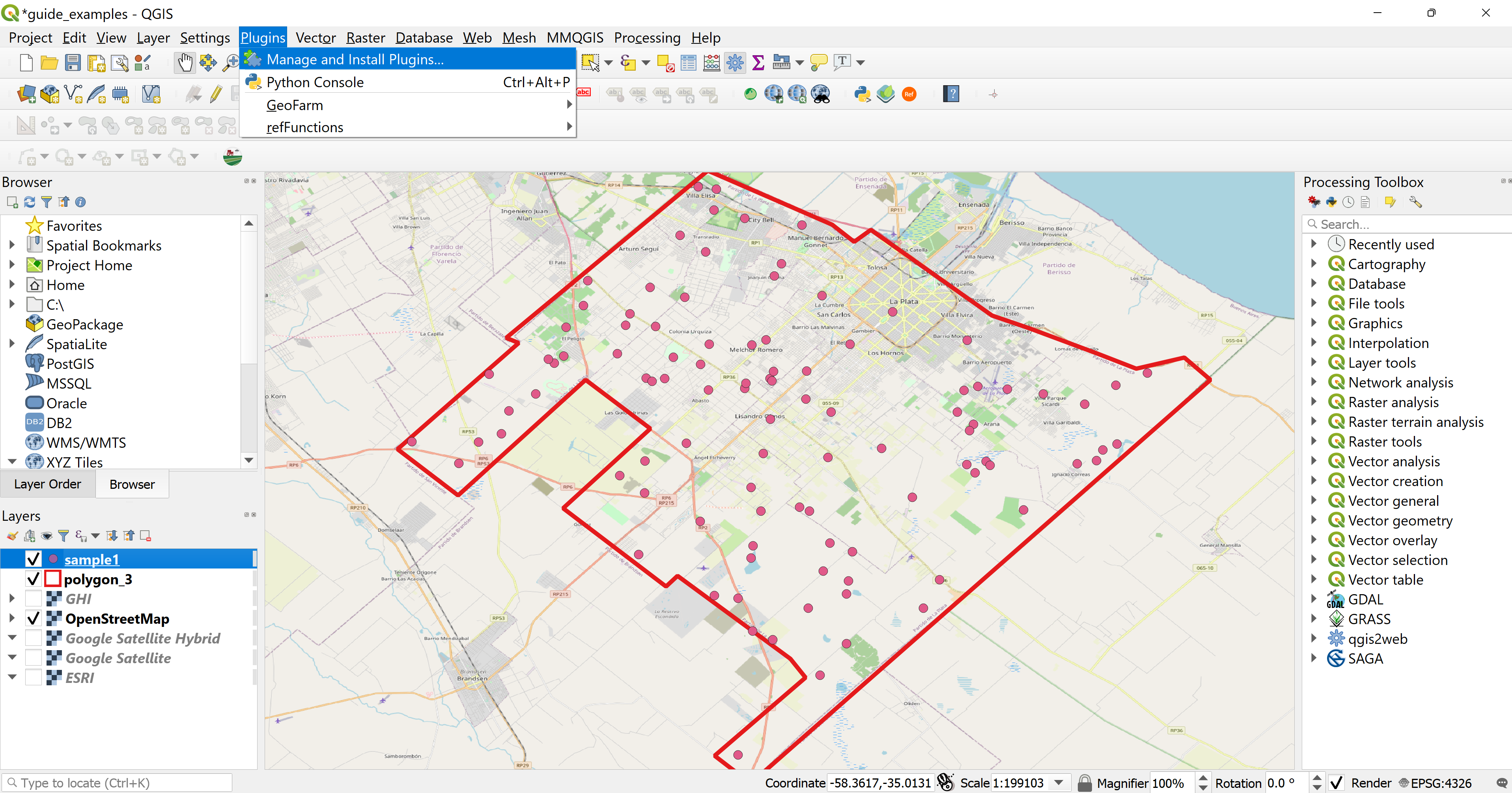
Figure 4.5: Plugins Menu

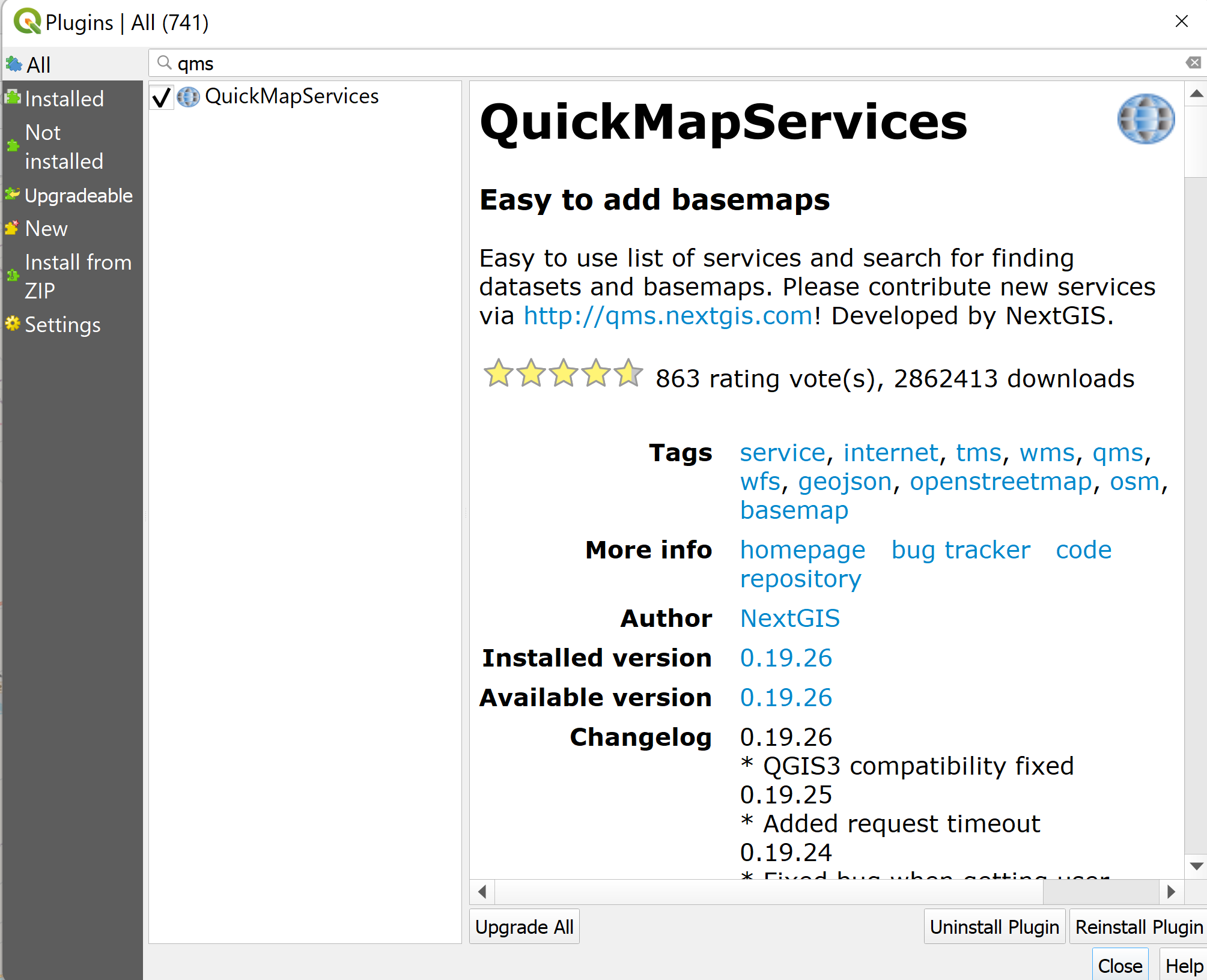
Figure 4.6: Plugins Dialog

To add the Search QMS panel we will right click on the menu bar and choose under Panels the Search QMS panel, the panel appears on the right side under the Processing Toolbox. In the search panel we can search for the QMS suitable for our project, here we see the QMS we need under the last used QMS, click add on the Google Satellite Hybrid and ESRI. (See 4.7 and 4.8)

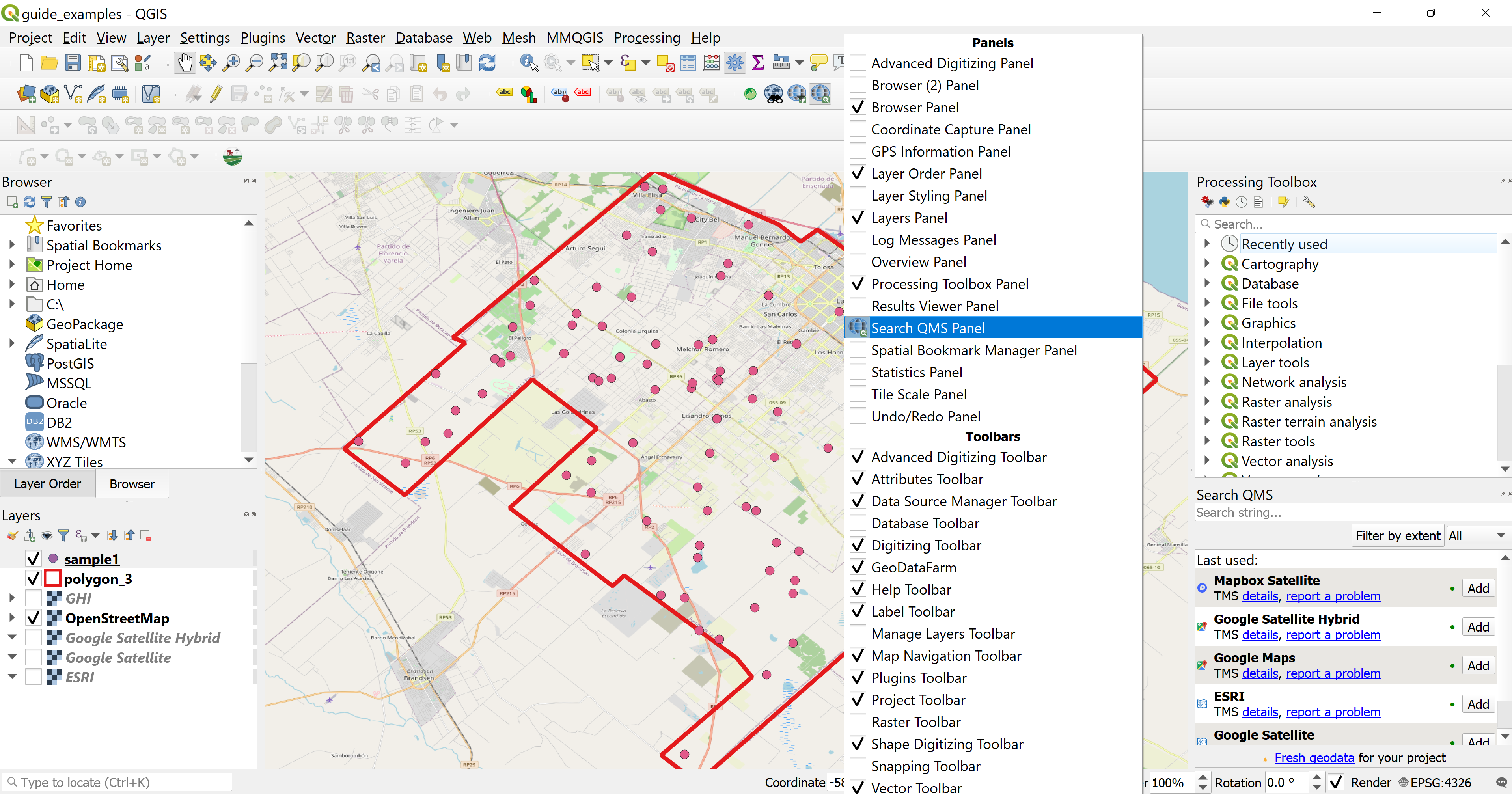
Figure 4.7: QMS Search Panel

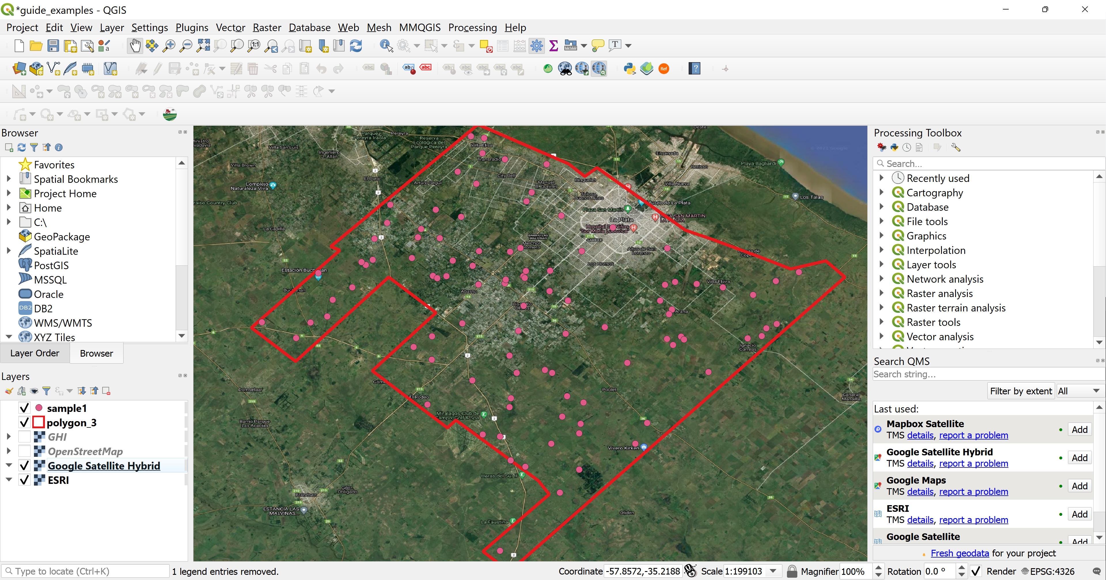
Figure 4.8: QMS in QGIS

4.2.2 Digitizing a sample with QMS

Now that we have the sample1 layer and QMS layers in our QGIS interface, the next step is to create a new polygon vector layer.
To do this we will go to the menu bar, click on the Layer Menu, select the Create Layer and there choose the New Shapefile Layer… option. (See 4.9)

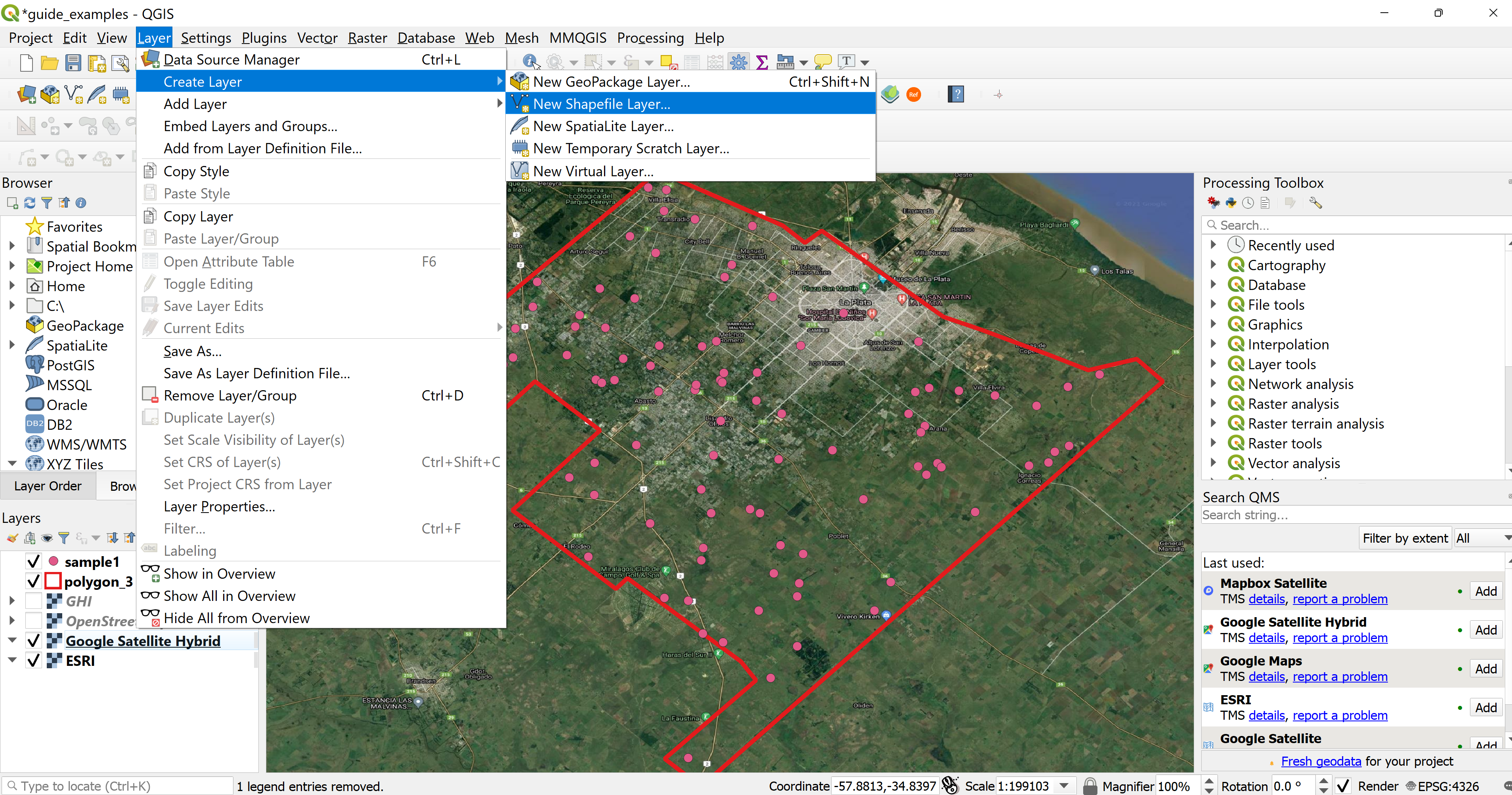
Figure 4.9: Create Vector Layer

The New Shapefile Layer… dialog will open and we can fill in the parameters for our layer. This layer we will name sample100. (See 4.10)

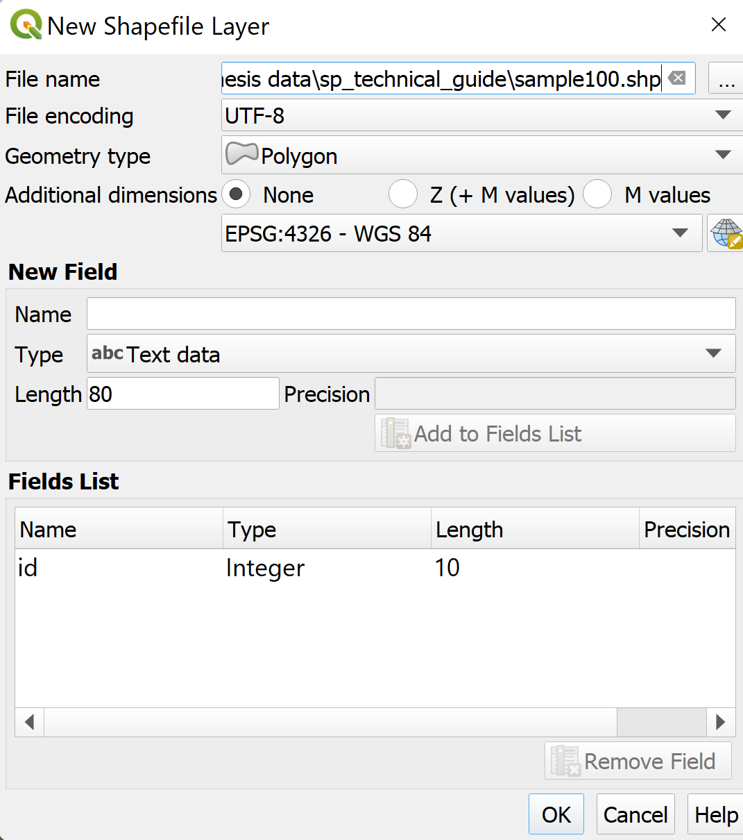
Figure 4.10: Create Vector Layer Dialog

Next we will right click on the sample100 layer and select the Toggle Editing option. This enables creating new polygons and adding them to the layer. Once the option is set we can see under the menu bar many different editing options in the Shape Digitizing Toolbar (if this is not already added, right click on the menu bar and select the toolbar under the Toolbars option), each time we want to digitize a new polygon we will click on the Add Polygon Feature option. (See 4.11 and 4.12)

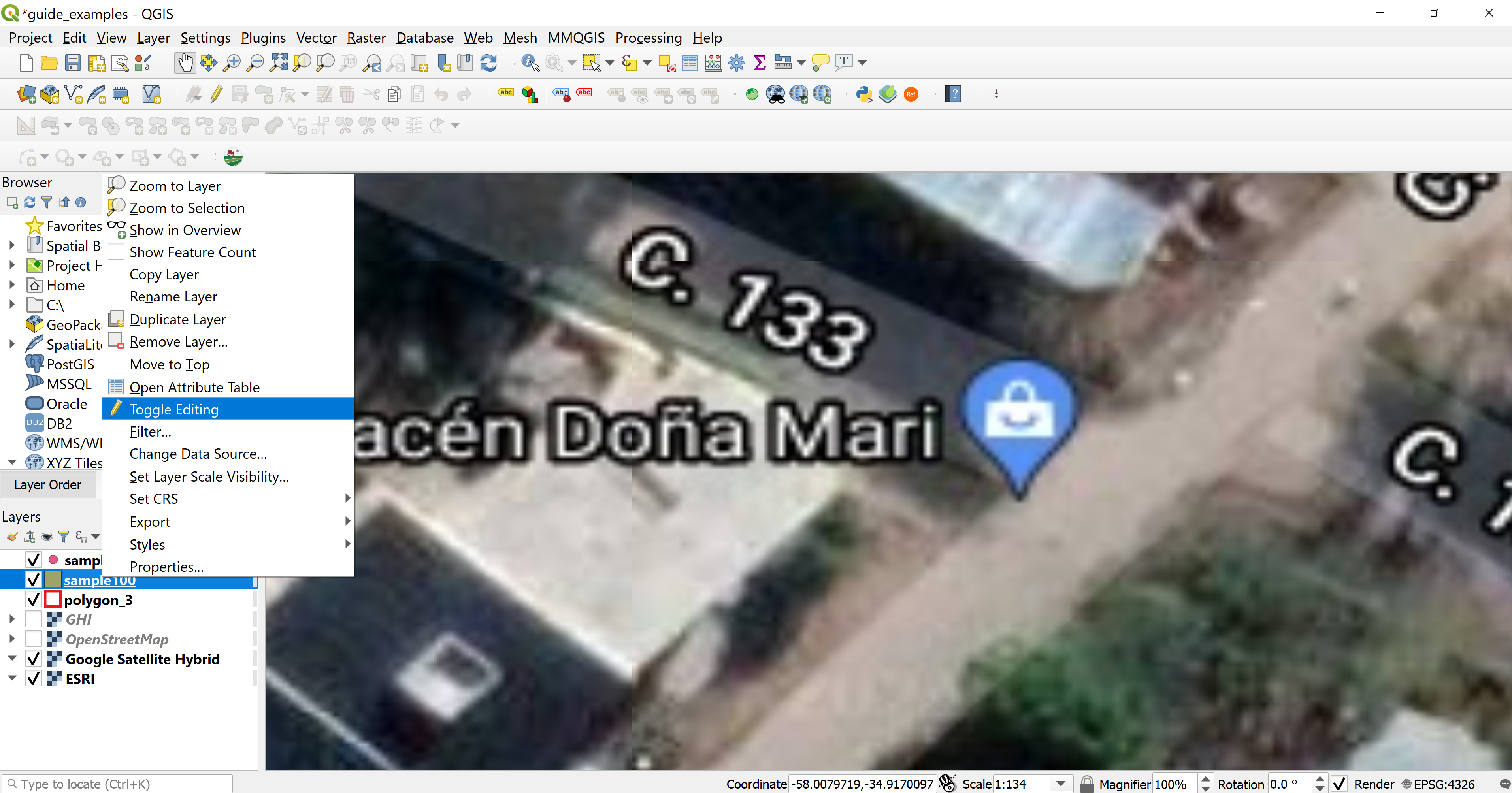
Figure 4.11: Toggle Editing

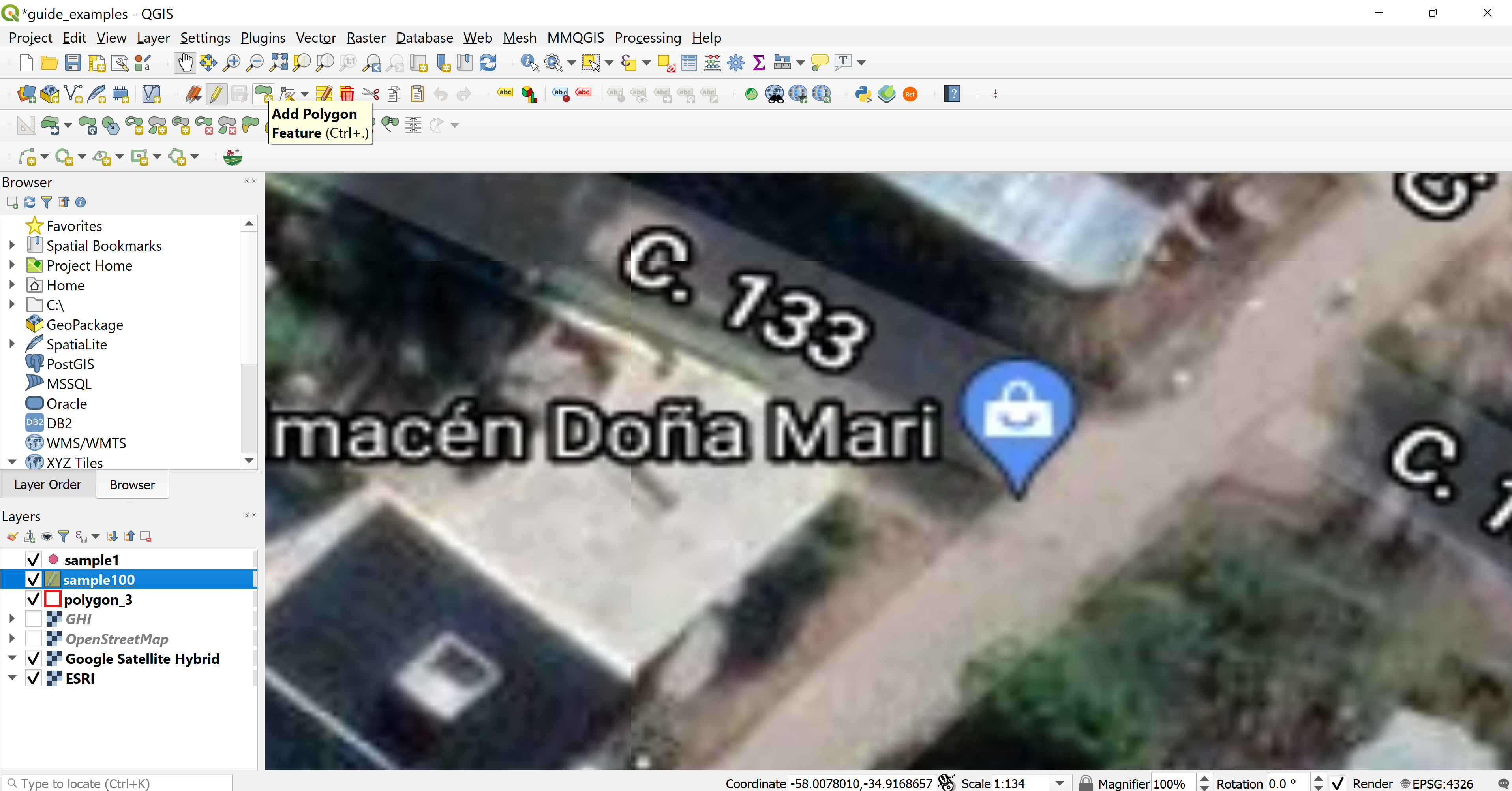
Figure 4.12: Shape Digitizing Toolbar - Add Polygon Feature

Once the layer sample100 is editable we will open the Attribute Table of sample1 and select a point according to the id field and click on the Zoom map to the selected rows option. We will see that the point id = 49, falls on a building rooftop. In 4.13 we see that id 49 is selected, it is recommended to start from the lowest id to the highest, to remember which point was already digitized.

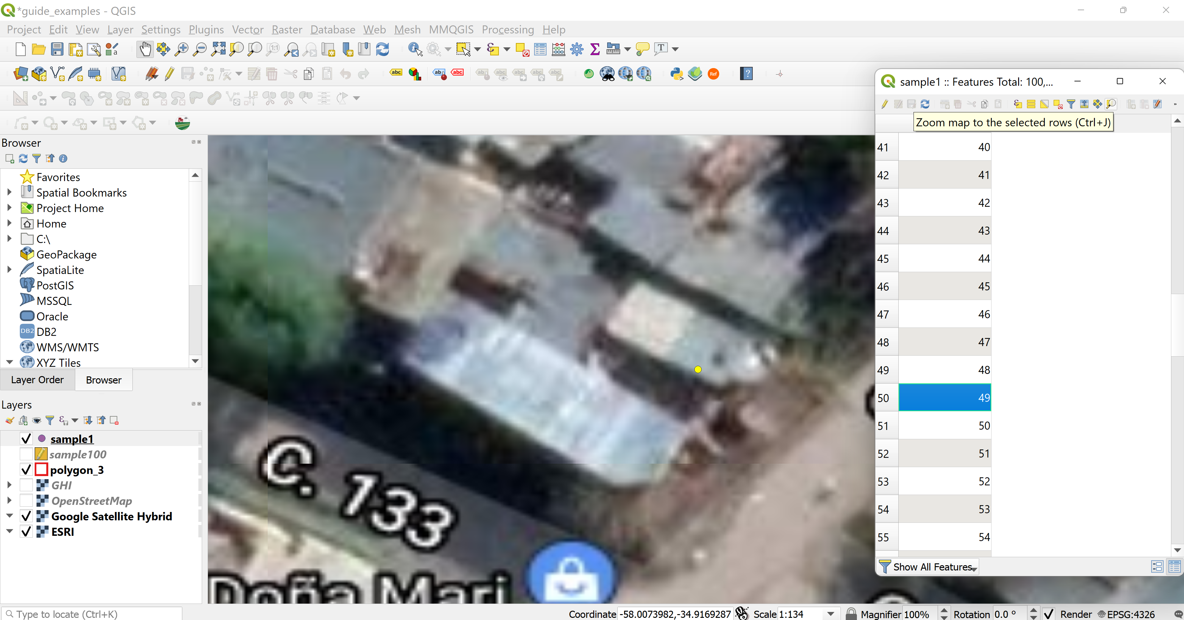
Figure 4.13: Random Point ID=49 from the layer sample1

Then we will click on the Add Polygon Feature option and follow the outline of the building rooftop using the TMS layers to achieve the best accuracy possible.(See 4.14)

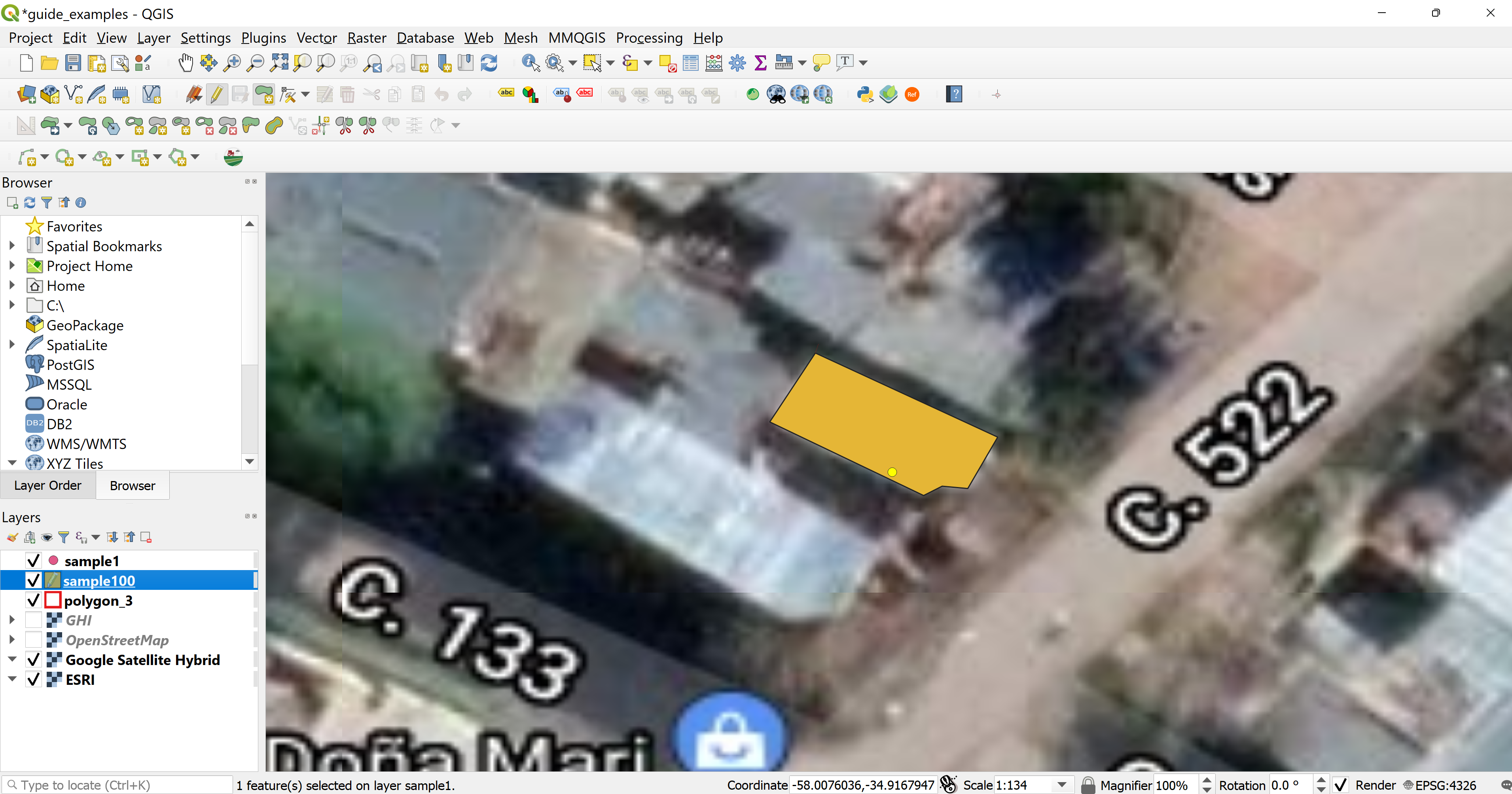
Figure 4.14: Digitizing ID=49 in the Layer sample100

For more information about digitizing and editing layers click here.

4.2.3 Including the density factor

Once a random point does not fall on a rooftop building we will digitize it to include it in our analysis as a density factor.
We will digitize the point in a small triangle shape, so the polygon’s area will be under 30 \(m^2\). (See 4.15)

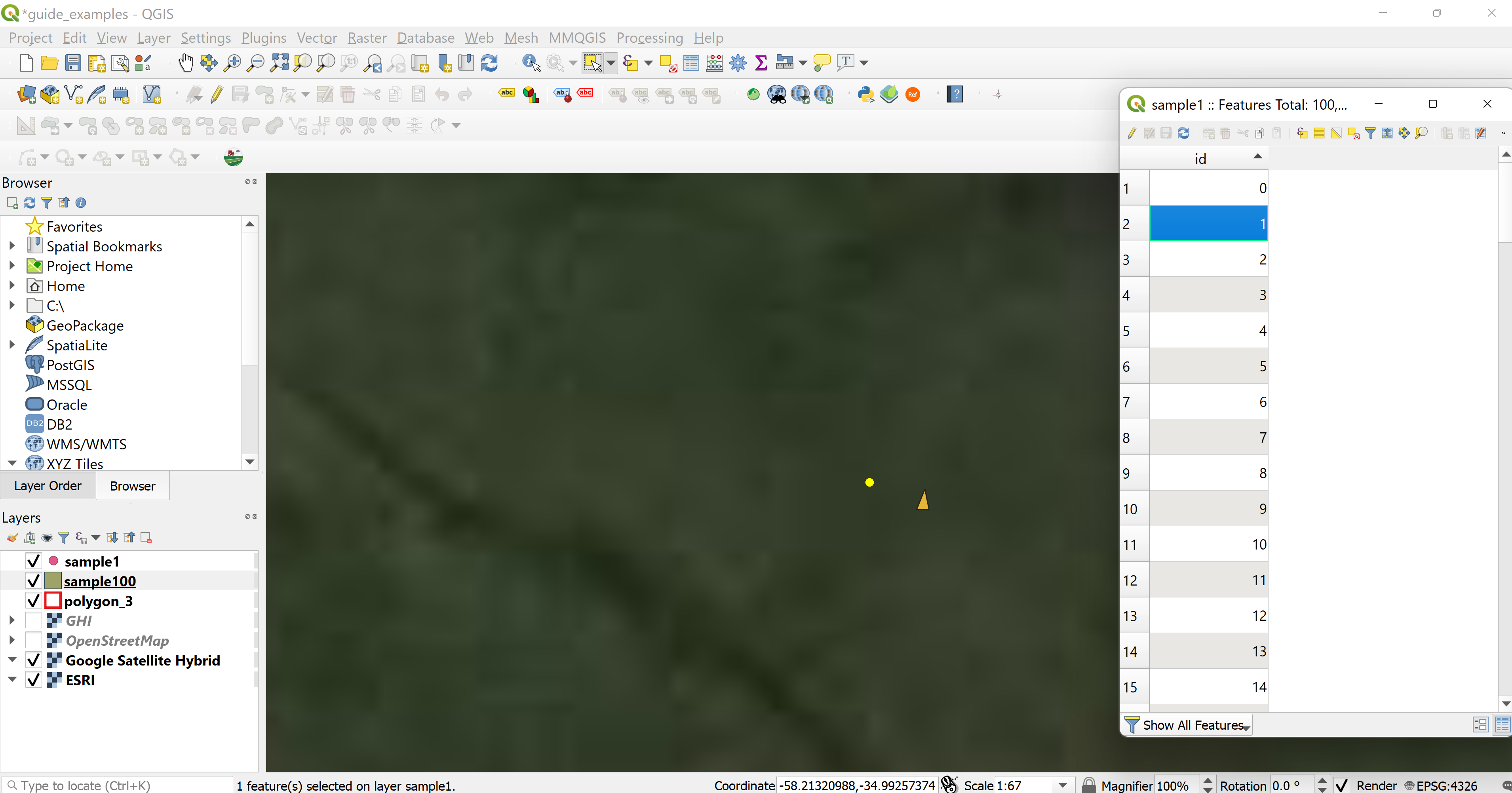
Figure 4.15: Digitizing to include the Density Factor

4.2.4 Solar radiation and renewable electricity calculation

Once finishing digitizing all the sample building rooftops, we will return to the steps described in chapter 3 and calculate the solar radiation and renewable electricity for the sample. (See 4.16)

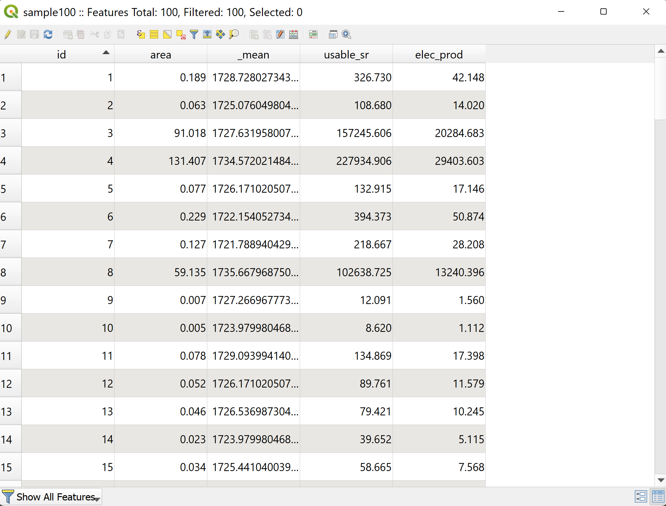
Figure 4.16: Sample100 Attribute Table with Calculations

As discussed in 4.1.1 we will digitize another sample for La Plata following the same steps as in 4.2.2 and 4.2.3, this time with 300 random points.