Chapter 13 VEC and VAR Models

rm(list=ls()) #Removes all items in Environment!
library(tseries) # for `adf.test()`
library(dynlm) #for function `dynlm()`
library(vars) # for function `VAR()`
library(nlWaldTest) # for the `nlWaldtest()` function
library(lmtest) #for `coeftest()` and `bptest()`.
library(broom) #for `glance(`) and `tidy()`
library(PoEdata) #for PoE4 datasets
library(car) #for `hccm()` robust standard errors
library(sandwich)
library(knitr) #for `kable()`
library(forecast) 

New package: vars (Pfaff 2013).

When there is no good reason to assume a one-way causal relationship between two time series variables we may think of their relationship as one of mutual interaction. The concept of “vector,” as in vector error correction refers to a number of series in such a model.

13.1 VAR and VEC Models

Equations $\ref{eq:var1defA13}$ and $\ref{eq:var1defA13}$ show a generic vector autoregression model of order 1, VAR(1), which can be estimated if the series are both I(0). If they are I(1), the same equations need to be estimated in first differences.

$$\begin{equation} y_{t}=\beta_{10}+\beta_{11}y_{t-1}+\beta_{12}x_{t-1}+\nu_{t}^y \label{eq:var1defA13} \end{equation}$$ $$\begin{equation} x_{t}=\beta_{20}+\beta_{21}y_{t-1}+\beta_{22}x_{t-1}+\nu_{t}^x \label{eq:var1defB13} \end{equation}$$

If the two variables in Equations $\ref{eq:var1defA13}$ and $\ref{eq:var1defB13}$ and are cointegrated, their cointegration relationship should be taken into account in the model, since it is valuable information; such a model is called vector error correction. The cointegration relationship is, remember, as shown in Equation $\ref{eq:gencointrelation13}$, where the error term has been proven to be stationary.

$$\begin{equation} y_{t}=\beta_{0}+\beta_{1}x_{t}+e_{t} \label{eq:gencointrelation13} \end{equation}$$

13.2 Estimating a VEC Model

The simplest method is a two-step procedure. First, estimate the cointegrating relationship given in Equation $\ref{eq:gencointrelation13}$ and created the lagged resulting residual series $\hat{e} _{t-1}=y_{t-1}-b_{0}-b_{1}x_{t-1}$. Second, estimate Equations $\ref{eq:ystep2VEC13}$ and $\ref{eq:xstep2VEC13}$ by OLS.

$$\begin{equation} \Delta y_{t}=\alpha_{10}+\alpha_{11}+\hat{e}_{t-1}+\nu_{t}^y \label{eq:ystep2VEC13} \end{equation}$$ $$\begin{equation} \Delta x_{t}=\alpha_{20}+\alpha_{21}+\hat{e}_{t-1}+\nu_{t}^x \label{eq:xstep2VEC13} \end{equation}$$

The following example uses the dataset $gdp$, which includes GDP series for Australia and USA for the period since 1970:1 to 2000:4. First we determine the order of integration of the two series.

data("gdp", package="PoEdata")
gdp <- ts(gdp, start=c(1970,1), end=c(2000,4), frequency=4)

ts.plot(gdp[,"usa"],gdp[,"aus"], type="l", 
        lty=c(1,2), col=c(1,2))
legend("topleft", border=NULL, legend=c("USA","AUS"), 
       lty=c(1,2), col=c(1,2))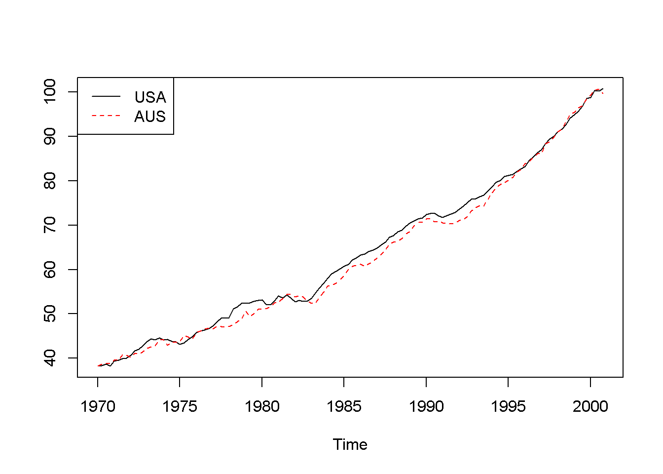

Figure 13.1: Australian and USA GDP series from dataset ‘gdp’

Figure 13.1 represents the two series in levels, revealing a common trend and, therefore, suggesting that the series are nonstationary.

adf.test(gdp[,"usa"])

## 
##  Augmented Dickey-Fuller Test
## 
## data:  gdp[, "usa"]
## Dickey-Fuller = -0.9083, Lag order = 4, p-value = 0.949
## alternative hypothesis: stationary

adf.test(gdp[,"aus"])

## 
##  Augmented Dickey-Fuller Test
## 
## data:  gdp[, "aus"]
## Dickey-Fuller = -0.6124, Lag order = 4, p-value = 0.975
## alternative hypothesis: stationary

adf.test(diff(gdp[,"usa"]))

## 
##  Augmented Dickey-Fuller Test
## 
## data:  diff(gdp[, "usa"])
## Dickey-Fuller = -4.293, Lag order = 4, p-value = 0.01
## alternative hypothesis: stationary

adf.test(diff(gdp[,"aus"]))

## 
##  Augmented Dickey-Fuller Test
## 
## data:  diff(gdp[, "aus"])
## Dickey-Fuller = -4.417, Lag order = 4, p-value = 0.01
## alternative hypothesis: stationary

The stationarity tests indicate that both series are I(1), Let us now test them for cointegration, using Equations $\ref{eq:au13}$ and $\ref{eq:eau13}$.

$$\begin{equation} aus_{t}=\beta_{1}usa_{t}+e_{t} \label{eq:au13} \end{equation}$$ $$\begin{equation} \hat{e}_{t}=aus_{t}-\beta_{1}usa_{t} \label{eq:eau13} \end{equation}$$

cint1.dyn <- dynlm(aus~usa-1, data=gdp)
kable(tidy(cint1.dyn), digits=3,
  caption="The results of the cointegration equation 'cint1.dyn'")

Table 13.1: The results of the cointegration equation ‘cint1.dyn’

term	estimate	std.error	statistic	p.value
usa	0.985	0.002	594.787	0

ehat <- resid(cint1.dyn)
cint2.dyn <- dynlm(d(ehat)~L(ehat)-1)
summary(cint2.dyn)

## 
## Time series regression with "ts" data:
## Start = 1970(2), End = 2000(4)
## 
## Call:
## dynlm(formula = d(ehat) ~ L(ehat) - 1)
## 
## Residuals:
##     Min      1Q  Median      3Q     Max 
## -1.4849 -0.3370 -0.0038  0.4656  1.3507 
## 
## Coefficients:
##         Estimate Std. Error t value Pr(>|t|)   
## L(ehat)  -0.1279     0.0443   -2.89   0.0046 **
## ---
## Signif. codes:  0 '***' 0.001 '**' 0.01 '*' 0.05 '.' 0.1 ' ' 1
## 
## Residual standard error: 0.598 on 122 degrees of freedom
## Multiple R-squared:  0.064,  Adjusted R-squared:  0.0564 
## F-statistic: 8.35 on 1 and 122 DF,  p-value: 0.00457

Our test rejects the null of no cointegration, meaning that the series are cointegrated. With cointegrated series we can construct a VEC model to better understand the causal relationship between the two variables.

vecaus<- dynlm(d(aus)~L(ehat), data=gdp)
vecusa <- dynlm(d(usa)~L(ehat), data=gdp)
tidy(vecaus)

term	estimate	std.error	statistic	p.value
(Intercept)	0.491706	0.057909	8.49094	0.000000
L(ehat)	-0.098703	0.047516	-2.07727	0.039893

tidy(vecusa)

term	estimate	std.error	statistic	p.value
(Intercept)	0.509884	0.046677	10.923715	0.000000
L(ehat)	0.030250	0.038299	0.789837	0.431168

The coefficient on the error correction term ($\hat{e}_{t-1}$) is significant for Australia, suggesting that changes in the US economy do affect Australian economy; the error correction coefficient in the US equation is not statistically significant, suggesting that changes in Australia do not influence American economy. To interpret the sign of the error correction coefficient, one should remember that $\hat{e}_{t-1}$ measures the deviation of Australian economy from its cointegrating level of $0.985$ of the US economy (see Equations $\ref{eq:au13}$ and $\ref{eq:eau13}$ and the value of $\beta_{1}$ in Table 13.1).

13.3 Estimating a VAR Model

The VAR model can be used when the variables under study are I(1) but not cointegrated. The model is the one in Equations $\ref{eq:var1def13}$, but in differences, as specified in Equations $\ref{eq:VARa13}$ and $\ref{eq:VARb13}$.

$$\begin{equation} \Delta y_{t}=\beta_{11}\Delta y_{t-1}+\beta_{12}\Delta x_{t-1}+\nu_{t}^{\Delta y} \label{eq:VARa13} \end{equation}$$ $$\begin{equation} \Delta x_{t}=\beta_{21}\Delta y_{t-1}+\beta_{22}\Delta x_{t-1}+\nu_{t}^{\Delta x} \label{eq:VARb13} \end{equation}$$

Let us look at the income-consumption relationship based on the $fred$ detaset, where consumption and income are already in logs, and the period is 1960:1 to 2009:4. Figure 13.2 shows that the two series both have a trend.

data("fred", package="PoEdata")
fred <- ts(fred, start=c(1960,1),end=c(2009,4),frequency=4)
ts.plot(fred[,"c"],fred[,"y"], type="l", 
        lty=c(1,2), col=c(1,2))
legend("topleft", border=NULL, legend=c("c","y"), 
       lty=c(1,2), col=c(1,2))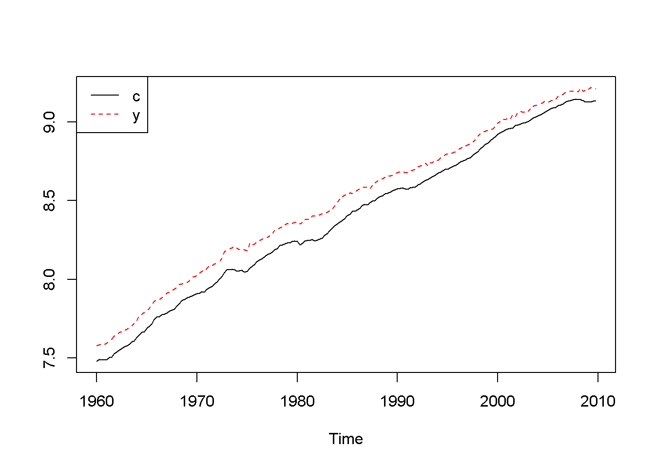

Figure 13.2: Logs of income (y) and consumption (c), dataset ‘fred’

Are the two series cointegrated?

Acf(fred[,"c"])
Acf(fred[,"y"])
adf.test(fred[,"c"])

## 
##  Augmented Dickey-Fuller Test
## 
## data:  fred[, "c"]
## Dickey-Fuller = -2.62, Lag order = 5, p-value = 0.316
## alternative hypothesis: stationary

adf.test(fred[,"y"])

## 
##  Augmented Dickey-Fuller Test
## 
## data:  fred[, "y"]
## Dickey-Fuller = -2.291, Lag order = 5, p-value = 0.454
## alternative hypothesis: stationary

adf.test(diff(fred[,"c"]))

## 
##  Augmented Dickey-Fuller Test
## 
## data:  diff(fred[, "c"])
## Dickey-Fuller = -4.713, Lag order = 5, p-value = 0.01
## alternative hypothesis: stationary

adf.test(diff(fred[,"y"]))

## 
##  Augmented Dickey-Fuller Test
## 
## data:  diff(fred[, "y"])
## Dickey-Fuller = -5.775, Lag order = 5, p-value = 0.01
## alternative hypothesis: stationary

cointcy <- dynlm(c~y, data=fred)
ehat <- resid(cointcy)
adf.test(ehat)

## 
##  Augmented Dickey-Fuller Test
## 
## data:  ehat
## Dickey-Fuller = -2.562, Lag order = 5, p-value = 0.341
## alternative hypothesis: stationary

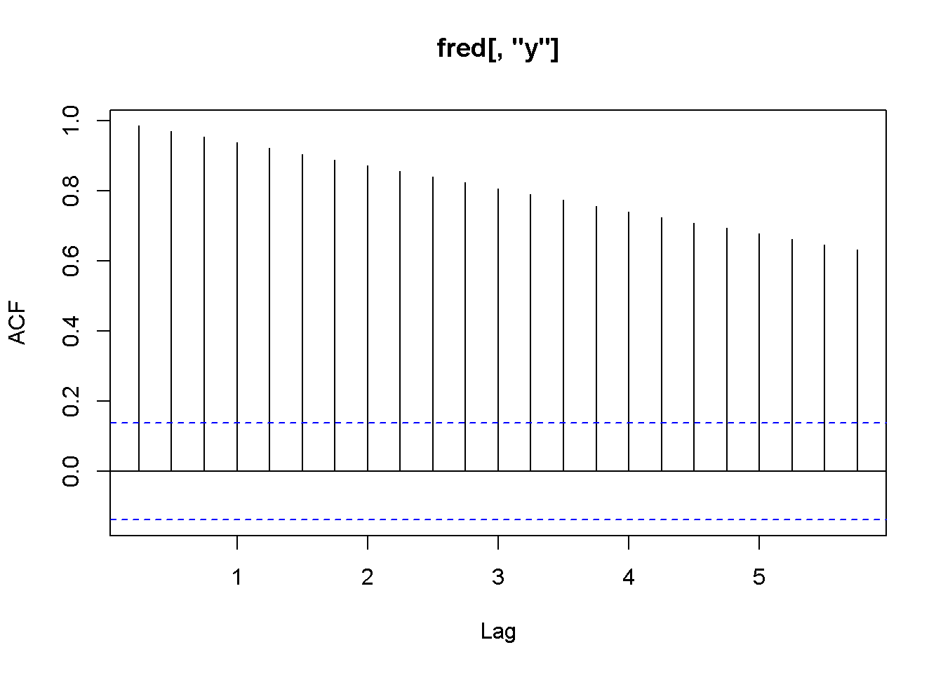
Figure 13.3: Correlograms for the series c and y, dataset fred

Figure 13.3 shows a long serial correlation sequence; therefore, I will let $R$ calculate the lag order in the ADF test. As the results of the above adf and cointegration tests show, the series are both I(1) but they fail the cointegration test (the series are not cointegrated.) (Plese rememebr that the adf.test function uses a constant and trend in the test equation; therefore, the critical values are not the same as in the textbook. However, the results of the tests should be the same most of the time.)

library(vars)
Dc <- diff(fred[,"c"])
Dy <- diff(fred[,"y"])
varmat <- as.matrix(cbind(Dc,Dy))
varfit <- VAR(varmat) # `VAR()` from package `vars`
summary(varfit)

## 
## VAR Estimation Results:
## ========================= 
## Endogenous variables: Dc, Dy 
## Deterministic variables: const 
## Sample size: 198 
## Log Likelihood: 1400.444 
## Roots of the characteristic polynomial:
## 0.344 0.343
## Call:
## VAR(y = varmat)
## 
## 
## Estimation results for equation Dc: 
## =================================== 
## Dc = Dc.l1 + Dy.l1 + const 
## 
##       Estimate Std. Error t value Pr(>|t|)    
## Dc.l1 0.215607   0.074749    2.88   0.0044 ** 
## Dy.l1 0.149380   0.057734    2.59   0.0104 *  
## const 0.005278   0.000757    6.97  4.8e-11 ***
## ---
## Signif. codes:  0 '***' 0.001 '**' 0.01 '*' 0.05 '.' 0.1 ' ' 1
## 
## 
## Residual standard error: 0.00658 on 195 degrees of freedom
## Multiple R-Squared: 0.12,    Adjusted R-squared: 0.111 
## F-statistic: 13.4 on 2 and 195 DF,  p-value: 3.66e-06 
## 
## 
## Estimation results for equation Dy: 
## =================================== 
## Dy = Dc.l1 + Dy.l1 + const 
## 
##        Estimate Std. Error t value Pr(>|t|)    
## Dc.l1  0.475428   0.097326    4.88  2.2e-06 ***
## Dy.l1 -0.217168   0.075173   -2.89   0.0043 ** 
## const  0.006037   0.000986    6.12  5.0e-09 ***
## ---
## Signif. codes:  0 '***' 0.001 '**' 0.01 '*' 0.05 '.' 0.1 ' ' 1
## 
## 
## Residual standard error: 0.00856 on 195 degrees of freedom
## Multiple R-Squared: 0.112,   Adjusted R-squared: 0.103 
## F-statistic: 12.3 on 2 and 195 DF,  p-value: 9.53e-06 
## 
## 
## 
## Covariance matrix of residuals:
##           Dc        Dy
## Dc 0.0000432 0.0000251
## Dy 0.0000251 0.0000733
## 
## Correlation matrix of residuals:
##       Dc    Dy
## Dc 1.000 0.446
## Dy 0.446 1.000

Function VAR(), which is part of the package vars (Pfaff 2013), accepts the following main arguments: y= a matrix containing the endogenous variables in the VAR model, p= the desired lag order (default is 1), and exogen= a matrix of exogenous variables. (VAR is a more powerful instrument than I imply here; please type ?VAR() for more information.) The results of a VAR model are more useful in analysing the time response to shocks in the variables, which is the topic of the next section.

13.4 Impulse Responses and Variance Decompositions

Impulse responses are best represented in graphs showing the responses of a VAR endogenous variable in time.

impresp <- irf(varfit)
plot(impresp)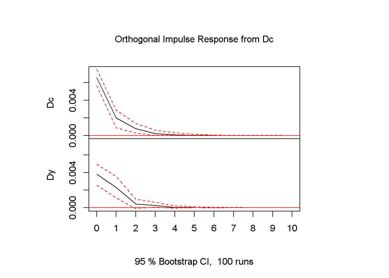

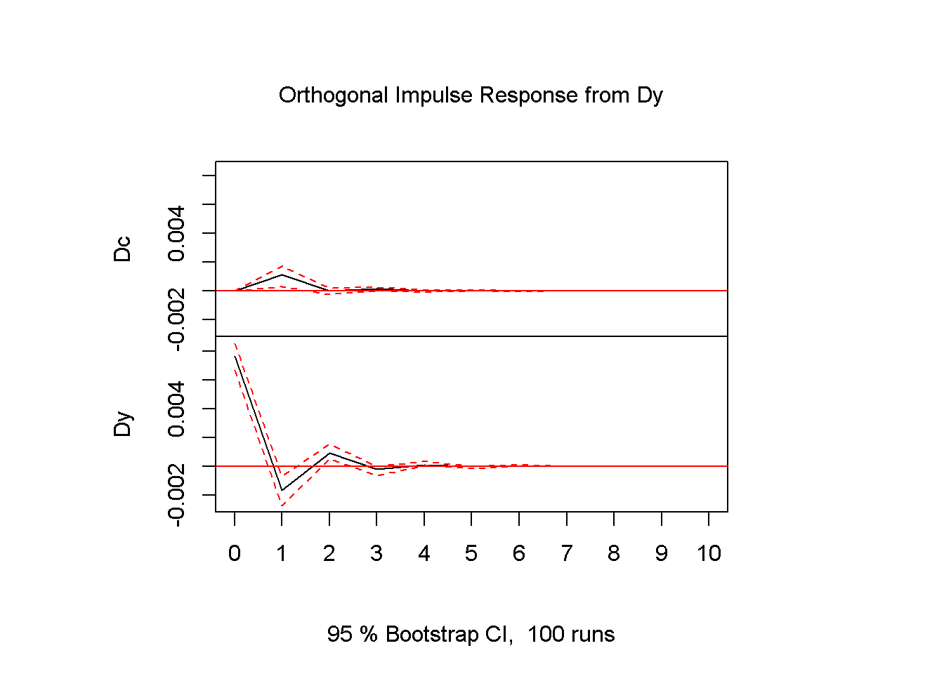
Figure 13.4: Impulse response diagrams for the series c and y, dataset fred

The interpretation of Figures 13.4 is straightforward: an impulse (shock) to $Dc$ at time zero has large effects the next period, but the effects become smaller and smaller as the time passes. The dotted lines show the 95 percent interval estimates of these effects. The VAR function prints the values corresponding to the impulse response graphs.

plot(fevd(varfit)) # `fevd()` is in package `vars`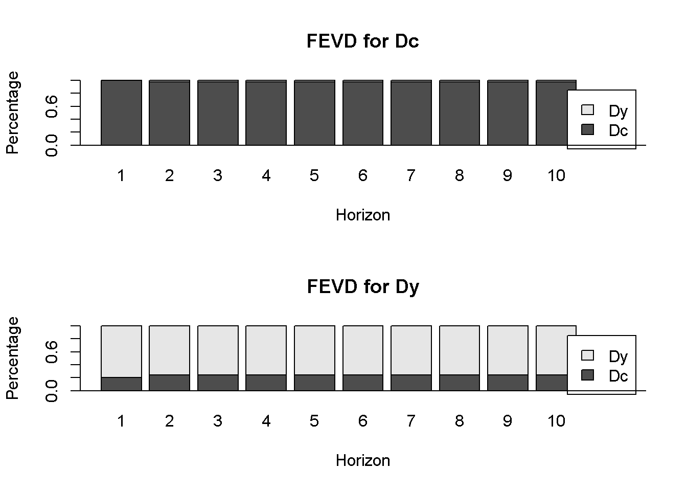

Figure 13.5: Forecast variance decomposition for the series c and y, dataset fred

Forecast variance decomposition estimates the contribution of a shock in each variable to the response in both variables. Figure 13.5 shows that almost 100 percent of the variance in $Dc$ is caused by $Dc$ itself, while only about 80 percent in the variance of $Dy$ is caused by $Dy$ and the rest is caused by $Dc$. The $R$ function fevd() in package vars allows forecast variance decomposition.

References

Pfaff, Bernhard. 2013. Vars: VAR Modelling. https://CRAN.R-project.org/package=vars.