Chapter 14 Time-Varying Volatility and ARCH Models
rm(list=ls()) #Removes all items in Environment!
library(FinTS) #for function `ArchTest()`
library(rugarch) #for GARCH models
library(tseries) # for `adf.test()`
library(dynlm) #for function `dynlm()`
library(vars) # for function `VAR()`
library(nlWaldTest) # for the `nlWaldtest()` function
library(lmtest) #for `coeftest()` and `bptest()`.
library(broom) #for `glance(`) and `tidy()`
library(PoEdata) #for PoE4 datasets
library(car) #for `hccm()` robust standard errors
library(sandwich)
library(knitr) #for `kable()`
library(forecast)
New packages: FinTS (Graves 2014) and rugarch (Ghalanos 2015).
The autoregressive conditional heteroskedasticity (ARCH) model concerns time series with time-varying heteroskedasticity, where variance is conditional on the information existing at a given point in time.
14.1 The ARCH Model
The ARCH model assumes that the conditional mean of the error term in a time series model is constant (zero), unlike the nonstationary series we have discussed so far), but its conditional variance is not. Such a model can be described as in Equations \ref{eq:archdefA14}, \ref{eq:archdefB14} and \ref{eq:archdefC14}.
\[\begin{equation} y_{t}=\phi +e_{t} \label{eq:archdefA14} \end{equation}\] \[\begin{equation} e_{t} | I_{t-1} \sim N(0,h_{t}) \label{eq:archdefB14} \end{equation}\] \[\begin{equation} h_{t}=\alpha_{0}+\alpha_{1}e_{t-1}^2, \;\;\;\alpha_{0}>0, \;\; 0\leq \alpha_{1}<1 \label{eq:archdefC14} \end{equation}\]Equations \ref{eq:archeffectseqA14} and \ref{eq:archeffectseqB14} give both the test model and the hypotheses to test for ARCH effects in a time series, where the residuals \(\hat e_{t}\) come from regressing the variable \(y_{t}\) on a constant, such as \ref{eq:archdefA14}, or on a constant plus other regressors; the test shown in Equation \ref{eq:archeffectseqA14} may include several lag terms, in which case the null hypothesis (Equation \ref{eq:archeffectseqB14}) would be that all of them are jointly insignificant.
\[\begin{equation} \hat e_{t}^2 = \gamma_{0}+\gamma_{1}\hat e_{t-1}^2+...+\gamma_{q}e_{t-q}^2+\nu_{t} \label{eq:archeffectseqA14} \end{equation}\] \[\begin{equation} H_{0}:\gamma_{1}=...=\gamma_{q}=0\;\;\;H_{A}:\gamma_{1}\neq 0\;or\;...\gamma_{q}\neq 0 \label{eq:archeffectseqB14} \end{equation}\]The null hypothesis is that there are no ARCH effects. The test statistic is \[(T-q)R^2 \sim \chi ^2_{(1-\alpha,q)}\]. The following example uses the dataset \(byd\), which contains 500 generated observations on the returns to shares in BrightenYourDay Lighting. Figure 14.1 shows a time series plot of the data and histogram.
data("byd", package="PoEdata")
rTS <- ts(byd$r)
plot.ts(rTS)
hist(rTS, main="", breaks=20, freq=FALSE, col="grey")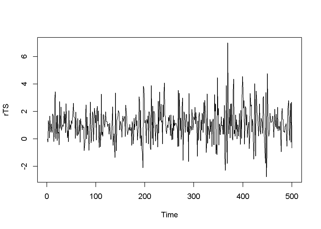
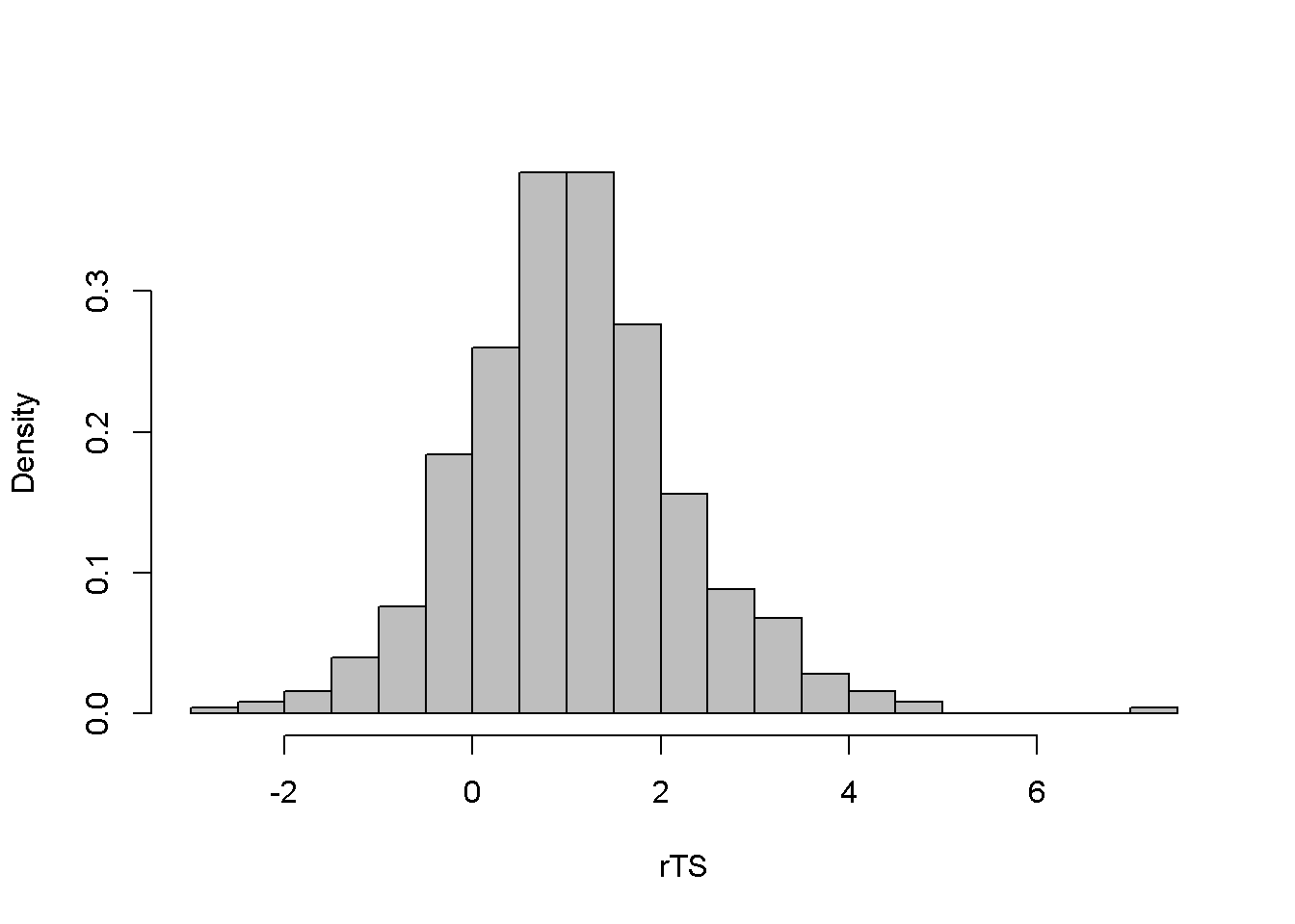
Figure 14.1: Level and histogram of variable ‘byd’
Let us first perform, step by step, the ARCH test described in Equations \ref{eq:archeffectseqA14} and \ref{eq:archeffectseqB14}, on the variable \(r\) from dataset \(byd\).
byd.mean <- dynlm(rTS~1)
summary(byd.mean)
##
## Time series regression with "ts" data:
## Start = 1, End = 500
##
## Call:
## dynlm(formula = rTS ~ 1)
##
## Residuals:
## Min 1Q Median 3Q Max
## -3.847 -0.723 -0.049 0.669 5.931
##
## Coefficients:
## Estimate Std. Error t value Pr(>|t|)
## (Intercept) 1.078 0.053 20.4 <2e-16 ***
## ---
## Signif. codes: 0 '***' 0.001 '**' 0.01 '*' 0.05 '.' 0.1 ' ' 1
##
## Residual standard error: 1.19 on 499 degrees of freedomehatsq <- ts(resid(byd.mean)^2)
byd.ARCH <- dynlm(ehatsq~L(ehatsq))
summary(byd.ARCH)##
## Time series regression with "ts" data:
## Start = 2, End = 500
##
## Call:
## dynlm(formula = ehatsq ~ L(ehatsq))
##
## Residuals:
## Min 1Q Median 3Q Max
## -10.802 -0.950 -0.705 0.320 31.347
##
## Coefficients:
## Estimate Std. Error t value Pr(>|t|)
## (Intercept) 0.908 0.124 7.30 1.1e-12 ***
## L(ehatsq) 0.353 0.042 8.41 4.4e-16 ***
## ---
## Signif. codes: 0 '***' 0.001 '**' 0.01 '*' 0.05 '.' 0.1 ' ' 1
##
## Residual standard error: 2.45 on 497 degrees of freedom
## Multiple R-squared: 0.125, Adjusted R-squared: 0.123
## F-statistic: 70.7 on 1 and 497 DF, p-value: 4.39e-16T <- nobs(byd.mean)
q <- length(coef(byd.ARCH))-1
Rsq <- glance(byd.ARCH)[[1]]
LM <- (T-q)*Rsq
alpha <- 0.05
Chicr <- qchisq(1-alpha, q)The result is the LM statistic, equal to \(62.16\), which is to be compared to the critical chi-squared value with \(\alpha =0.05\) and \(q=1\) degrees of freedom; this value is \(\chi^2 _{(0.95,1)}=3.84\); this indicates that the null hypothesis is rejected, concluding that the series has ARCH effects.
The same conclusion can be reached if, instead of the step-by-step procedure we use one of \(R\)’s ARCH test capabilities, the ArchTest() function in package FinTS.
bydArchTest <- ArchTest(byd, lags=1, demean=TRUE)
bydArchTest
##
## ARCH LM-test; Null hypothesis: no ARCH effects
##
## data: byd
## Chi-squared = 62.16, df = 1, p-value = 3.22e-15Function garch() in the tseries package, becomes an ARCH model when used with the order= argument equal to c(0,1). This function can be used to estimate and plot the variance \(h_{t}\) defined in Equation \ref{eq:archdefC14}, as shown in the following code and in Figure 14.2.
byd.arch <- garch(rTS,c(0,1))##
## ***** ESTIMATION WITH ANALYTICAL GRADIENT *****
##
##
## I INITIAL X(I) D(I)
##
## 1 1.334069e+00 1.000e+00
## 2 5.000000e-02 1.000e+00
##
## IT NF F RELDF PRELDF RELDX STPPAR D*STEP NPRELDF
## 0 1 5.255e+02
## 1 2 5.087e+02 3.20e-02 7.13e-01 3.1e-01 3.8e+02 1.0e+00 1.34e+02
## 2 3 5.004e+02 1.62e-02 1.78e-02 1.2e-01 1.9e+00 5.0e-01 2.11e-01
## 3 5 4.803e+02 4.03e-02 4.07e-02 1.2e-01 2.1e+00 5.0e-01 1.42e-01
## 4 7 4.795e+02 1.60e-03 1.99e-03 1.3e-02 9.7e+00 5.0e-02 1.36e-02
## 5 8 4.793e+02 4.86e-04 6.54e-04 1.2e-02 2.3e+00 5.0e-02 2.31e-03
## 6 9 4.791e+02 4.16e-04 4.93e-04 1.2e-02 1.7e+00 5.0e-02 1.39e-03
## 7 10 4.789e+02 3.80e-04 4.95e-04 2.3e-02 4.6e-01 1.0e-01 5.36e-04
## 8 11 4.789e+02 6.55e-06 6.73e-06 9.0e-04 0.0e+00 5.1e-03 6.73e-06
## 9 12 4.789e+02 4.13e-08 3.97e-08 2.2e-04 0.0e+00 9.8e-04 3.97e-08
## 10 13 4.789e+02 6.67e-11 6.67e-11 9.3e-06 0.0e+00 4.2e-05 6.67e-11
##
## ***** RELATIVE FUNCTION CONVERGENCE *****
##
## FUNCTION 4.788831e+02 RELDX 9.327e-06
## FUNC. EVALS 13 GRAD. EVALS 11
## PRELDF 6.671e-11 NPRELDF 6.671e-11
##
## I FINAL X(I) D(I) G(I)
##
## 1 2.152304e+00 1.000e+00 -2.370e-06
## 2 1.592050e-01 1.000e+00 -7.896e-06sbydarch <- summary(byd.arch)
sbydarch##
## Call:
## garch(x = rTS, order = c(0, 1))
##
## Model:
## GARCH(0,1)
##
## Residuals:
## Min 1Q Median 3Q Max
## -1.459 0.220 0.668 1.079 4.293
##
## Coefficient(s):
## Estimate Std. Error t value Pr(>|t|)
## a0 2.1523 0.1857 11.59 <2e-16 ***
## a1 0.1592 0.0674 2.36 0.018 *
## ---
## Signif. codes: 0 '***' 0.001 '**' 0.01 '*' 0.05 '.' 0.1 ' ' 1
##
## Diagnostic Tests:
## Jarque Bera Test
##
## data: Residuals
## X-squared = 48.57, df = 2, p-value = 2.85e-11
##
##
## Box-Ljung test
##
## data: Squared.Residuals
## X-squared = 0.1224, df = 1, p-value = 0.726hhat <- ts(2*byd.arch$fitted.values[-1,1]^2)
plot.ts(hhat)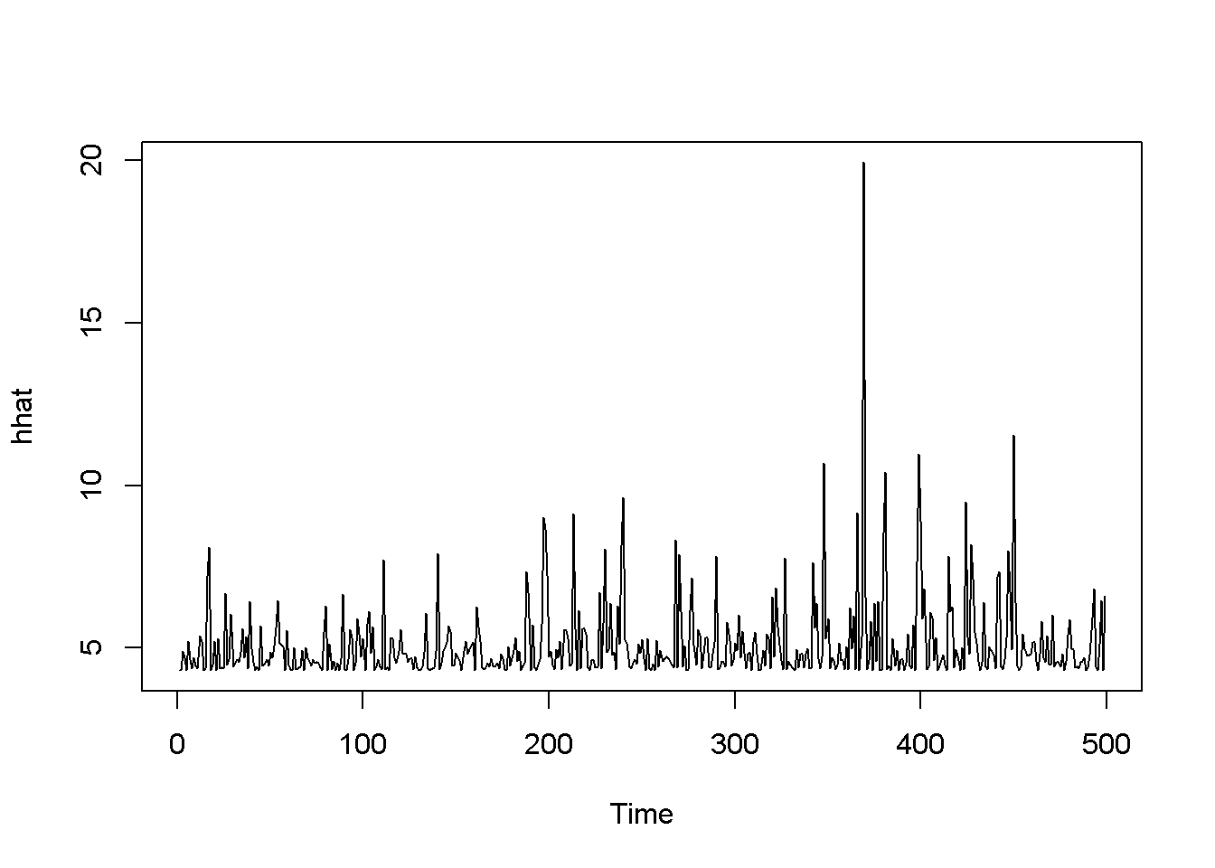
Figure 14.2: Estimated ARCH(1) variance for the ‘byd’ dataset
14.2 The GARCH Model
# Using package `rugarch` for GARCH models
library(rugarch)
garchSpec <- ugarchspec(
           variance.model=list(model="sGARCH",
                               garchOrder=c(1,1)),
           mean.model=list(armaOrder=c(0,0)),
           distribution.model="std")
garchFit <- ugarchfit(spec=garchSpec, data=rTS)
coef(garchFit)
## mu omega alpha1 beta1 shape
## 1.049280 0.396544 0.495161 0.240827 99.999225rhat <- garchFit@fit$fitted.values
plot.ts(rhat)
hhat <- ts(garchFit@fit$sigma^2)
plot.ts(hhat)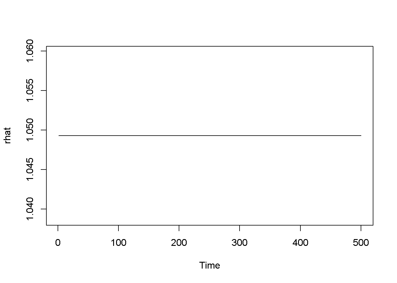
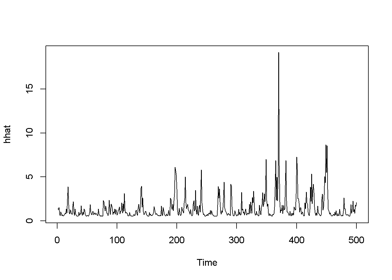
Figure 14.3: Standard GARCH model (sGARCH) with dataset ‘byd’
# tGARCH
garchMod <- ugarchspec(variance.model=list(model="fGARCH",
                               garchOrder=c(1,1),
                               submodel="TGARCH"),
           mean.model=list(armaOrder=c(0,0)),
           distribution.model="std")
garchFit <- ugarchfit(spec=garchMod, data=rTS)
coef(garchFit)
## mu omega alpha1 beta1 eta11 shape
## 0.986682 0.352207 0.390636 0.375328 0.339432 99.999884rhat <- garchFit@fit$fitted.values
plot.ts(rhat)
hhat <- ts(garchFit@fit$sigma^2)
plot.ts(hhat)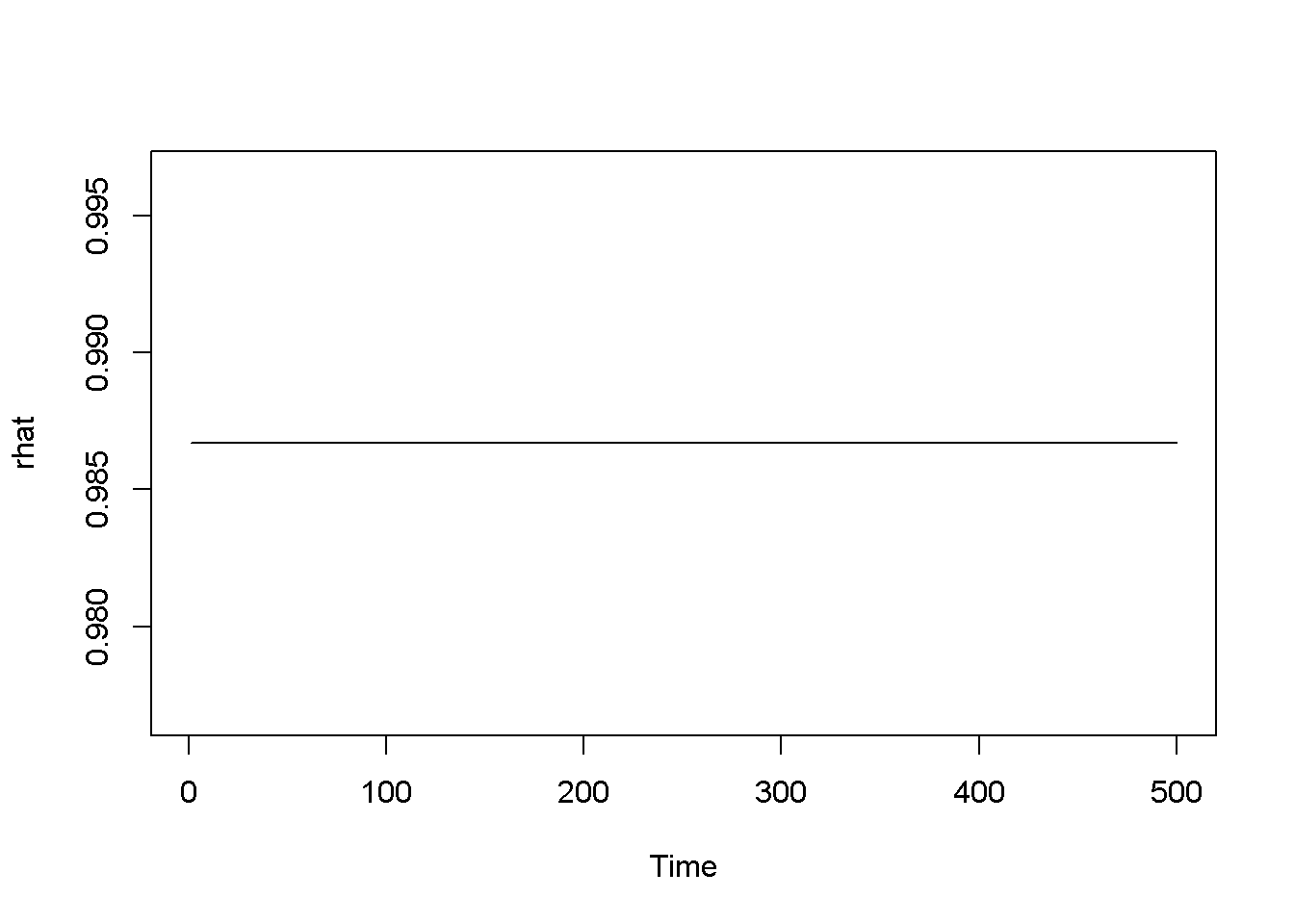
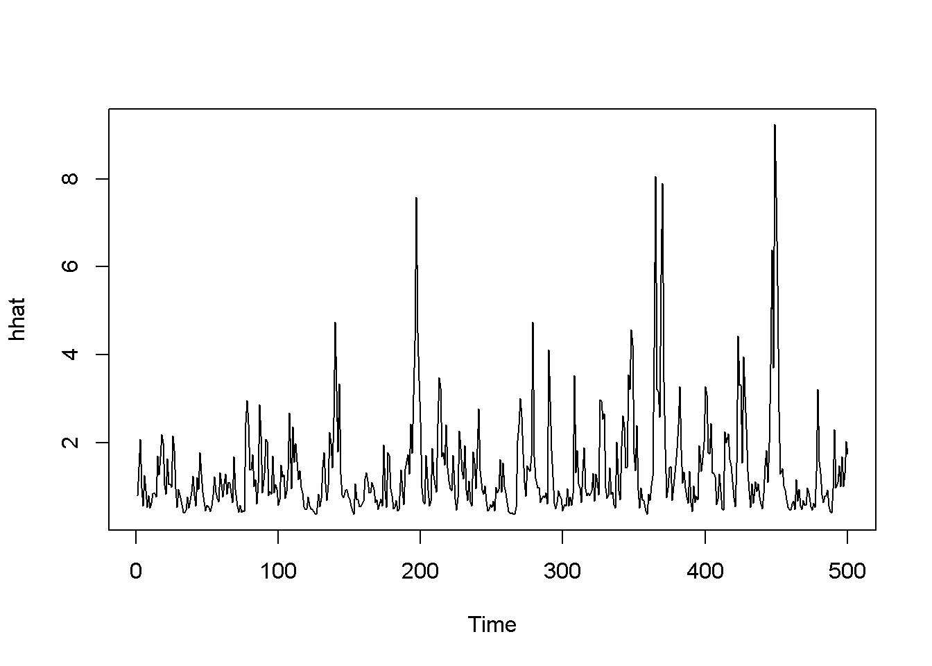
Figure 14.4: The tGARCH model with dataset ‘byd’
# GARCH-in-mean
garchMod <- ugarchspec(
          variance.model=list(model="fGARCH",
                               garchOrder=c(1,1),
                               submodel="APARCH"),
           mean.model=list(armaOrder=c(0,0),
                          include.mean=TRUE,
                          archm=TRUE,
                          archpow=2
                          ),
           distribution.model="std"
                           )
garchFit <- ugarchfit(spec=garchMod, data=rTS)
coef(garchFit)
## mu archm omega alpha1 beta1 eta11
## 0.820603 0.193476 0.368730 0.442930 0.286748 0.185531
## lambda shape
## 1.897586 100.000000rhat <- garchFit@fit$fitted.values
plot.ts(rhat)
hhat <- ts(garchFit@fit$sigma^2)
plot.ts(hhat)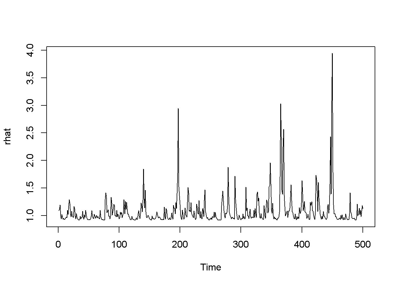

Figure 14.5: A version of the GARCH-in-mean model with dataset ‘byd’
Figures 14.3, 14.4, and 14.5 show a few versions of the GARCH model. Predictions can be obtained using the function ugarchboot() from the package ugarch.
References
Graves, Spencer. 2014. FinTS: Companion to Tsay (2005) Analysis of Financial Time Series. https://CRAN.R-project.org/package=FinTS.
Ghalanos, Alexios. 2015. Rugarch: Univariate Garch Models. https://CRAN.R-project.org/package=rugarch.