Chapter 3 Interval Estimation and Hypothesis Testing
library(xtable)
library(PoEdata)
library(knitr)
So far we estimated only a number for a regression parameter such as \(\beta_{2}\). This estimate, however, gives no indication of its reliablity, since it is just a realization of the random variable \(b_{2}\). An interval estimate, which is also known as a confidence interval is an interval centerd on an estimated value, which includes the true parameter with a given probability, say 95%. A coefficient of the linear regression model such as \(b_{2}\) is normally distributed with its mean equal to the population parameter \(\beta_{2}\) and a variance that depends on the population variance \(\sigma^2\) and the sample size:
\[\begin{equation} b_{2}\sim N \left(\beta_{2},\; \frac{\sigma^2}{\sum(x_{i}-\bar{x})^2}\right), \label{eq:normb23} \end{equation}\]3.1 The Estimated Distribution of Regression Coefficients
Equation \ref{eq:normb23} gives the theoretical distribution of a linear regression coefficient, a distribution that is not very useful since it requires the unknown population variance \(\sigma^2\). If we replace \(\sigma^2\) with an estimated variance \(\hat\sigma^2\) given in Equation \ref{eq:sighat13}, the standardized distribution of \(b_{2}\) becomes a \(t\) distribution with \(N-2\) degrees of freedom.
\[\begin{equation} \hat{\sigma}^2=\frac{\sum \hat{e}_{i}^2}{N-2} \label{eq:sighat13} \end{equation}\]Equation \ref{eq:tratio31} shows the the \(t\)-ratio:
\[\begin{equation} t=\frac{b_{2}-\beta_{2}}{se(b_{2})} \label{eq:tratio31} \end{equation}\]3.2 Confidence Interval in General
An interval estimate of \(b_{2}\) based on the \(t\)-ratio is calculated in Equation \ref{eq:intest31}, which we can consider as “an interval that includes the true parameter \(\beta_{2}\) with a probability of \(100(1-\alpha)\%\).” In this context, \(\alpha\) is called significance level, and the interval is called, for example, a 95% confidence interval estimate for \(\beta_{2}\). The critical value of the \(t\)-ratio, \(t_{c}\), depends on the chosen significance level and on the number of degrees of freedom. In \(R\), the function that returns critical values for the \(t\) distribution is \(qt(1-\frac{ \alpha }{2}, df)\), where \(df\) is the number of degrees of freedom.
\[\begin{equation} b_{2}\pm t_{c}\times se(b_{2}) \label{eq:intest31} \end{equation}\]A side note about using distributions in \(R\). There are four types of functions related to distributions, each type’s name beginning with one of the following four letters: p for the cummulative distribution function, d for density, r for a draw of a random number from the respective distribution, and q for quantile. This first letter is followed by a few letters suggesting what distribution we refer to, such as norm, t, f, and chisq. Now, if we put toghether the first letter and the distribution name, we get functions such as the following, where x and q stand for quantiles, p stands for probability, df is degree of freedom (of which \(F\) has two), n is the desired number of draws, and lower.tail can be TRUE (default) if probabilities are \(P[X \le x]\) or FALSE if probabilities are \(P[X>x]\):
For the uniform distribution:
- dunif(x, min = 0, max = 1)
- punif(q, min = 0, max = 1, lower.tail = TRUE)
- qunif(p, min = 0, max = 1, lower.tail = TRUE)
- runif(n, min = 0, max = 1)
For the normal distribution:
- dnorm(x, mean = 0, sd = 1)
- pnorm(q, mean = 0, sd = 1, lower.tail = TRUE)
- qnorm(p, mean = 0, sd = 1, lower.tail = TRUE)
- rnorm(n, mean = 0, sd = 1)
For the \(t\) distribution:
- dt(x, df)
- pt(q, df, lower.tail = TRUE)
- qt(p, df, lower.tail = TRUE)
- rt(n, df)
For the \(F\) distribution:
- df(x, df1, df2)
- pf(q, df1, df2, lower.tail = TRUE)
- qf(p, df1, df2, lower.tail = TRUE)
- rf(n, df1, df2)
For the \(\chi^2\) distribution:
- dchisq(x, df)
- pchisq(q, df, lower.tail = TRUE)
- qchisq(p, df, lower.tail = TRUE)
- rchisq(n, df)
3.3 Example: Confidence Intervals in the food Model
Let us calculate a 95% confidence interval for the coefficient on \(income\) in the food expenditure model. Besides coalculating confidence intervals, the following lines of code demonstratre how to retrieve information such as standard errors of coefficients from the summary() output. The function summary summarizes the results of a linear regression, some of which are not available directly from running the model itself.
library(PoEdata)
data("food")
alpha <- 0.05 # chosen significance level
mod1 <- lm(food_exp~income, data=food)
b2 <- coef(mod1)[[2]]
df <- df.residual(mod1) # degrees of freedom
smod1 <- summary(mod1)
seb2 <- coef(smod1)[2,2] # se(b2)
tc <- qt(1-alpha/2, df)
lowb <- b2-tc*seb2  # lower bound
upb <- b2+tc*seb2   # upper bound
The resulting confidence interval for the coefficient \(b_{2}\) in the food simple regression model is \((5.97, 14.45)\).
R has a special function, confint(model), that can calculate confidence intervals taking as its argument the name of a regression model. The result of applying this function is a \(K \times 2\) matrix with a confidence interval (two values: lower and upper bound) on each row and a number of lines equal to the number of parametrs in the model (equal to 2 in the simple linear regression model). Compare the values from the next code to the ones from the previous to check that they are equal.
ci <- confint(mod1)
print(ci)
## 2.5 % 97.5 %
## (Intercept) -4.46328 171.2953
## income 5.97205 14.4472lowb_b2 <- ci[2, 1] # lower bound
upb_b2 <- ci[2, 2] # upper bound. 3.4 Confidence Intervals in Repeated Samples
data("table2_2")
alpha <- 0.05
mod1 <- lm(y1~x, data=table2_2) # just to determine df
tc <- qt(1-alpha/2, df) # critical t

# Initiate four vectors that will store the results:
lowb1 <- rep(0, 10) # 'repeat 0 ten times'
upb1 <- rep(0, 10)  # (alternatively, 'numeric(10)')
lowb2 <- rep(0, 10)
upb2 <-rep(0, 10)

# One loop for each set of income:
for(i in 2:11){  # The curly bracket begins the loop
  dat <- data.frame(cbind(table2_2[,1], table2_2[,i]))
  names(dat) <- c("x", "y")
  mod1 <- lm(y~x, data=dat)
  smod1 <- summary(mod1)
  b1 <- coef(mod1)[[1]]
  b2 <- coef(mod1)[[2]]
  seb1 <- coef(smod1)[1,2]
  seb2 <- coef(smod1)[2,2]
  lowb1[i-1] <- b1-tc*seb1
  upb1[i-1] <- b1+tc*seb1
  lowb2[i-1] <- b2-tc*seb2
  upb2[i-1] <- b2+tc*seb2
} # This curly bracket ends the loop

table <- data.frame(lowb1, upb1, lowb2, upb2)
kable(table,
  caption="Confidence intervals for $b_{1}$ and $b_{2}$",
align="c")| lowb1 | upb1 | lowb2 | upb2 |
|---|---|---|---|
| 49.542182 | 213.846 | 2.51843 | 10.4413 |
| -9.831097 | 124.323 | 7.64838 | 14.1174 |
| 28.556681 | 179.264 | 4.50553 | 11.7727 |
| -20.959444 | 113.968 | 8.64817 | 15.1545 |
| 0.931168 | 167.534 | 5.27120 | 13.3049 |
| -66.044847 | 119.302 | 9.08188 | 18.0194 |
| -0.629753 | 129.046 | 7.80618 | 14.0592 |
| 19.194721 | 140.129 | 6.84889 | 12.6804 |
| 38.315701 | 156.287 | 5.20631 | 10.8950 |
| 20.691744 | 171.232 | 4.13968 | 11.3988 |
Table 3.1 shows the lower and upper bounds of the confidence intervals of \(\beta_{1}\) and \(\beta_{2}\).
3.5 Hypothesis Tests
Hypothesis testing seeks to establish whether the data sample at hand provides sufficient evidence to support a certain conjecture (hypothesis) about a population parameter such as the intercept in a regresion model, the slope, or some combination of them. The procedure requires three elements: the hypotheses (the null and the alternative), a test statistic, which in the case of the simple linear regression parameters is the t-ratio, and a significance level, \(\alpha\).
Suppose we believe that there is a significant relationship between a household’s income and its expenditure on food, a conjecture which has led us to formulate the food expenditure model in the first place. Thus, we believe that \(\beta_{2}\), the (population) parameter, is different from zero. Equation \ref{eq:hytst1} shows the null and alternative hypotheses for such a test.
\[\begin{equation} H_{0}:\beta_{2}=0, \; \; \; \; H_{A}:\beta_{2} \neq 0 \label{eq:hytst1} \end{equation}\]In general, if a null hypothesis \(H_{0}: \beta_{k}=c\) is true, the t statistic (the t-ratio) is given by Equation \ref{eq:tstat} and has a t distribution with \(N-2\) degrees of freedom.
\[\begin{equation} t=\frac{b_{k}-c}{se(b_{k})}\sim t_{(N-2)} \label{eq:tstat} \end{equation}\]Let us test the hypothesis in Equation \ref{eq:hytst1}, which makes \(c=0\) in Equation \ref{eq:tstat}. Let \(\alpha=0.05\). Table 3.2 shows the regression output.
alpha <- 0.05
library(PoEdata); library(xtable); library(knitr)
data("food")
mod1 <- lm(food_exp~income, data=food)
smod1 <- summary(mod1)
table <- data.frame(xtable(mod1))
kable(table,
caption="Regression output showing the coefficients")| Estimate | Std..Error | t.value | Pr…t.. | |
|---|---|---|---|---|
| (Intercept) | 83.4160 | 43.41016 | 1.92158 | 0.062182 |
| income | 10.2096 | 2.09326 | 4.87738 | 0.000019 |
b2 <- coef(mod1)[["income"]] #coefficient on income
# or:
b2 <- coef(mod1)[[2]] # the coefficient on income
seb2 <- sqrt(vcov(mod1)[2,2]) #standard error of b2
df <- df.residual(mod1) # degrees of freedom
t <- b2/seb2
tcr <- qt(1-alpha/2, df)
The results \(t=\) \(4.88\) and \(t_{cr}=\) \(2.02\) show that \(t>t_{cr}\), and therefore \(t\) falls in the rejection region (see Figure 3.1).
# Plot the density function and the values of t:
curve(dt(x, df), -2.5*seb2, 2.5*seb2, ylab=" ", xlab="t")
abline(v=c(-tcr, tcr, t), col=c("red", "red", "blue"),
       lty=c(2,2,3))
legend("topleft", legend=c("-tcr", "tcr", "t"), col=
         c("red", "red", "blue"), lty=c(2, 2, 3))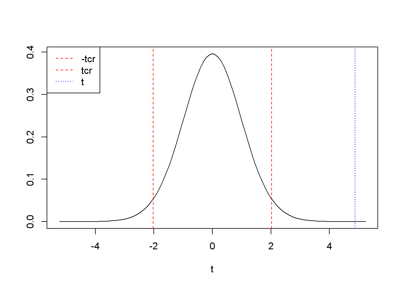
Figure 3.1: A two-tail hypothesis testing for \(b_{2}\) in the \(food\) example
Suppose we are interested to determine if \(\beta_{2}\) is greater than 5.5. This conjecture will go into the alternative hypothesis: \(H_{0}\le 5.5, \; \; \; H_{A}>5.5\). The procedure is the same as for the two-tail test, but now the whole rejection region is to the right of the critical value \(t_{cr}\).
c <- 5.5
alpha <- 0.05
t <- (b2-c)/seb2
tcr <- qt(1-alpha, df) # note: alpha is not divided by 2
curve(dt(x, df), -2.5*seb2, 2.5*seb2, ylab=" ", xlab="t")
abline(v=c(tcr, t), col=c("red", "blue"), lty=c(2, 3))
legend("topleft", legend=c("tcr", "t"),
       col=c("red", "blue"), lty=c(2, 3))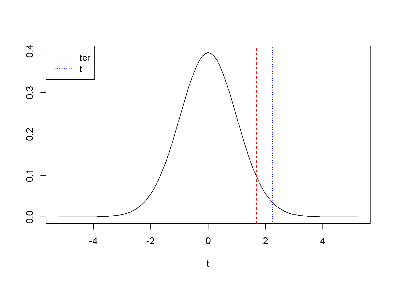
Figure 3.2: Right-tail test: the rejection region is to the right of \(t_{cr}\)
Figure 3.2 shows \(t_{cr}=\) \(1.685954\), \(t= 2.249904\). Since \(t\) falls again in the rejection region, we can reject the null hypothesis \(H_{0}: \beta_{2}\le 0\).
A left-tail test is not different from the right-tail one, but of course the rejection region is to the left of \(t_{cr}\). For example, if we are interested to determine if \(\beta_{2}\) is less than 15, we place this conjecture in the alternative hypothesis: \(H_{0} \ge 15, \; \; \; H_{A}<15\). The novelty here is how we use the qt() function to calculate \(t_{cr}\): instead of qt(1-alpha, ...), we need to use qt(alpha, ...). Figure 3.3 illustrates this example, where the rejection region is, remember, to the left of \(t_{cr}\).
c <- 15
alpha <- 0.05
t <- (b2-c)/seb2
tcr <- qt(alpha, df) # note: alpha is not divided by 2
curve(dt(x, df), -2.5*seb2, 2.5*seb2, ylab=" ", xlab="t")
abline(v=c(tcr, t), col=c("red", "blue"), lty=c(2, 3))
legend("topleft", legend=c("tcr", "t"),
       col=c("red", "blue"), lty=c(2, 3))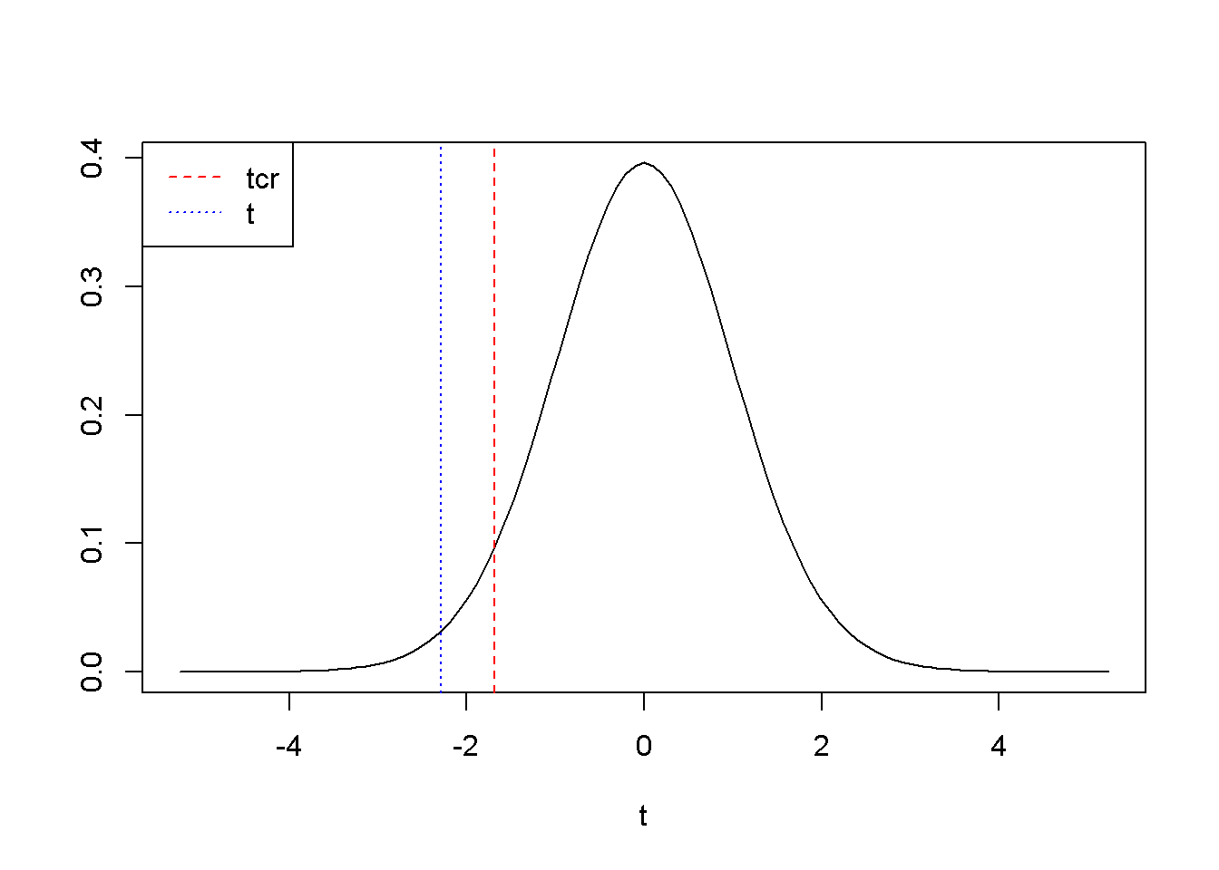
Figure 3.3: Left-tail test: the rejection region is to the left of \(t_{cr}=\)
R does automatically a test of significance, which is indeed testing the hypothesis \(H_{0}: \beta_{2}=0, \; \; \; H_{A}: \beta_{2} \ne 0\). The regression output shows the values of the \(t\)-ratio for all the regression coefficients.
library(PoEdata)
data("food")
mod1 <- lm(food_exp ~ income, data = food)
table <- data.frame(round(xtable(summary(mod1)), 3))
kable(table, caption = "Regression output for the 'food' model")| Estimate | Std..Error | t.value | Pr…t.. | |
|---|---|---|---|---|
| (Intercept) | 83.416 | 43.410 | 1.922 | 0.062 |
| income | 10.210 | 2.093 | 4.877 | 0.000 |
Table 3.3 shows the regression output where the \(t\)-statistics of the coefficients can be observed.
3.6 The p-Value
In the context of a hypothesis test, the \(p\)-value is the area outside the calculated \(t\)-statistic; it is the probability that the \(t\)-ratio takes a value that is more extreme than the calculated one, under the assumption that the null hypothesis is true. We reject the null hypothesis if the \(p\)-value is less than a chosen significance level. For a right-tail test, the \(p\)-value is the area to the right of the calculated \(t\); for a left-tail test it is the area to the left of the calculated \(t\); for a two-tail test the \(p\)-value is split in two equal amounts: \(p/2\) to the left and \(p/2\) to the right. \(p\)-values are calculated in \(R\) by the function pt(t, df), where \(t\) is the calculated \(t\)-ratio and \(df\) is the number of degrees of freedom in the estimated model.
Right-tail test, \(H_{0}:\beta_{2}\le c, \; \; \; H_{A}: \beta_{2}>c\).
# Calculating the p-value for a right-tail test
c <- 5.5
t <- (b2-c)/seb2
p <- 1-pt(t, df) # pt() returns p-values;
The right-tail test shown in Figure 3.2 gives the \(p\)-value \(p=0.01516\).
Left-tail test, \(H_{0}:\beta_{2}\ge c, \; \; \; H_{A}: \beta_{2}<c\).
# Calculating the p-value for a left-tail test
c <- 15
t <- (b2-c)/seb2
p <- pt(t, df)
The left-tail test shown in Figure 3.3 gives the \(p\)-value \(p=\) \(0.01388\).
Two-tail test, \(H_{0}:\beta_{2}= c, \; \; \; H_{A}: \beta_{2}\ne c\).
# Calculating the p-value for a two-tail test
c <- 0
t <- (b2-c)/seb2
p <- 2*(1-pt(abs(t), df))
The two-tail test shown in Figure 3.4 gives the \(p\)-value \(p=\) \(2\times 10^{-5}\), for a \(t\)-ratio \(t=\) \(4.88\).
curve(dt(x, df), from=-2.5*seb2, to=2.5*seb2)
abline(v=c(-t, t), col=c("blue", "blue"), lty=c(2, 2))
legend("topright", legend=c("-t", "t"),
       col=c("blue", "blue"), lty=c(2, 4))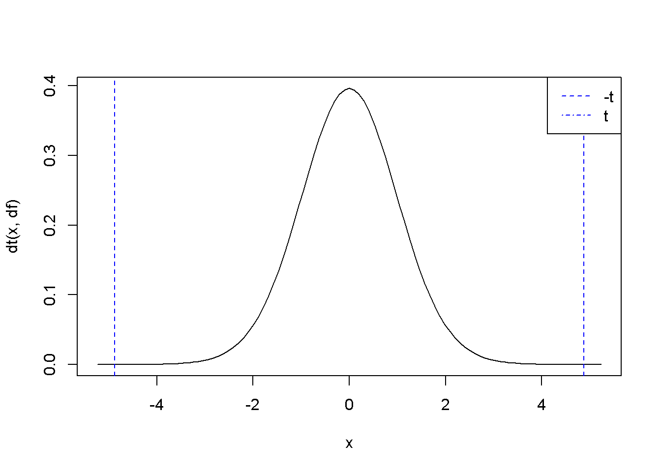
Figure 3.4: The \(p\)-value in two-tail hypothesis testing
R gives the \(p\)-values in the standard regression output, which we can retrieve using the summary(model) function. Table 3.4 shows the output of the regression model, where the \(p\)-values can be observed.
table <- data.frame(xtable(smod1))
knitr::kable(table, caption=
"Regression output showing p-values")| Estimate | Std..Error | t.value | Pr…t.. | |
|---|---|---|---|---|
| (Intercept) | 83.4160 | 43.41016 | 1.92158 | 0.062182 |
| income | 10.2096 | 2.09326 | 4.87738 | 0.000019 |
3.7 Testing Linear Combinations of Parameters
Sometimes we wish to estimate the expected value of the dependent variable, \(y\), for a given value of \(x\). For example, according to our food model, what is the average expenditure of a household having income of $2000? We need to estimate the linear combination of the regression coefficients \(\beta_{1}\) and \(\beta_{2}\) given in Equation \ref{eq:lincombfood} (let’s denote the linear combination by \(L\)).
\[\begin{equation} L=E(food\_exp | income=20)=\beta_{1} + 20 \beta_{2} \label{eq:lincombfood} \end{equation}\]Finding confidence intervals and testing hypotheses about the linear combination in Equation \ref{eq:lincombfood} requires calculating a \(t\)-statistic similar to the one for the regression coefficients we calculated before. However, estimating the standard error of the linear combination is not as straightforward. In general, if \(X\) and \(Y\) are two random variables and \(a\) and \(b\) two constants, the variance of the linear combination \(aX+bY\) is
\[\begin{equation} var( aX+bY) =a^2var(X)+b^2var(Y)+2abcov(X,Y). \label{eq:vargen} \end{equation}\]Now, let us apply the formula in Equation \ref{eq:vargen} to the linear combination of \(\beta{1}\) and \(\beta{2}\) given by Equation \ref{eq:lincombfood}, we obtain Equation \ref{eq:varfood}.
\[\begin{equation} var( b_{1}+20 b_{2})=var(b_{1})+20^2var(b_{2})+2 \times 20cov(b_{1} b_{2}) \label{eq:varfood} \end{equation}\]The following sequence of code determines an interval estimate for the expected value of food expenditure in a household earning $2000 a week.
library(PoEdata)
data("food")
alpha <- 0.05
x <- 20 # income is in 100s, remember?
m1 <- lm(food_exp~income, data=food)
tcr <- qt(1-alpha/2, df) # rejection region right of tcr.
df <- df.residual(m1)
b1 <- m1$coef[1]
b2 <- m1$coef[2]
varb1 <- vcov(m1)[1, 1]
varb2 <- vcov(m1)[2, 2]
covb1b2 <- vcov(m1)[1, 2]
L <- b1+b2*x  # estimated L
varL = varb1 + x^2 * varb2 + 2*x*covb1b2 # var(L)
seL <- sqrt(varL) # standard error of L
lowbL <- L-tcr*seL
upbL <- L+tcr*seL
The result is the confidence interval (\(258.91\), \(316.31\)). Next, we test hypotheses about the linear combination \(L\) defined in Equation \ref{eq:lincombfood}, looking at the three types of hypotheses: two-tail, left-tail, and right-tail. Equations \ref{eq:lineartest31e} \(-\) \ref{eq:lineartest33e} show the test setups for a hypothesized value of food expenditure \(c\).
\[\begin{equation} H_{0}: L=c, \; \; \; H_{A}:L\ne c \label{eq:lineartest31e} \end{equation}\] \[\begin{equation} H_{0}: L\ge c, \; \; \; H_{A}:L < c \label{eq:lineartest32e} \end{equation}\] \[\begin{equation} H_{0}: L\le c, \; \; \; H_{A}:L > c \label{eq:lineartest33e} \end{equation}\]One should use the function pt(t, df) carefully, because it gives wrong results when testing hypotheses using the \(p\)-value metod and the calculated \(t\) is negative. Therefore, the absolute value of \(t\) should be used. Figure 3.5 shows the \(p\)-values calculated with the formula 1-pt(t, df). When \(t\) is positive and the test is two-tail, doubling the \(p\)-value 1-pt(t, df) is correct; but when \(t\) is negative, the correct \(p\)-value is 2*p(t, df).
.shadenorm(above=1.6, justabove=TRUE)
segments(1.6,0,1.6,0.2,col="blue", lty=3)
legend("topleft", legend="t", col="blue", lty=3)

.shadenorm(above=-1.6, justabove=TRUE)
segments(-1.6,0,-1.6,0.2,col="blue", lty=3)
legend("topleft", legend="t", col="blue", lty=3)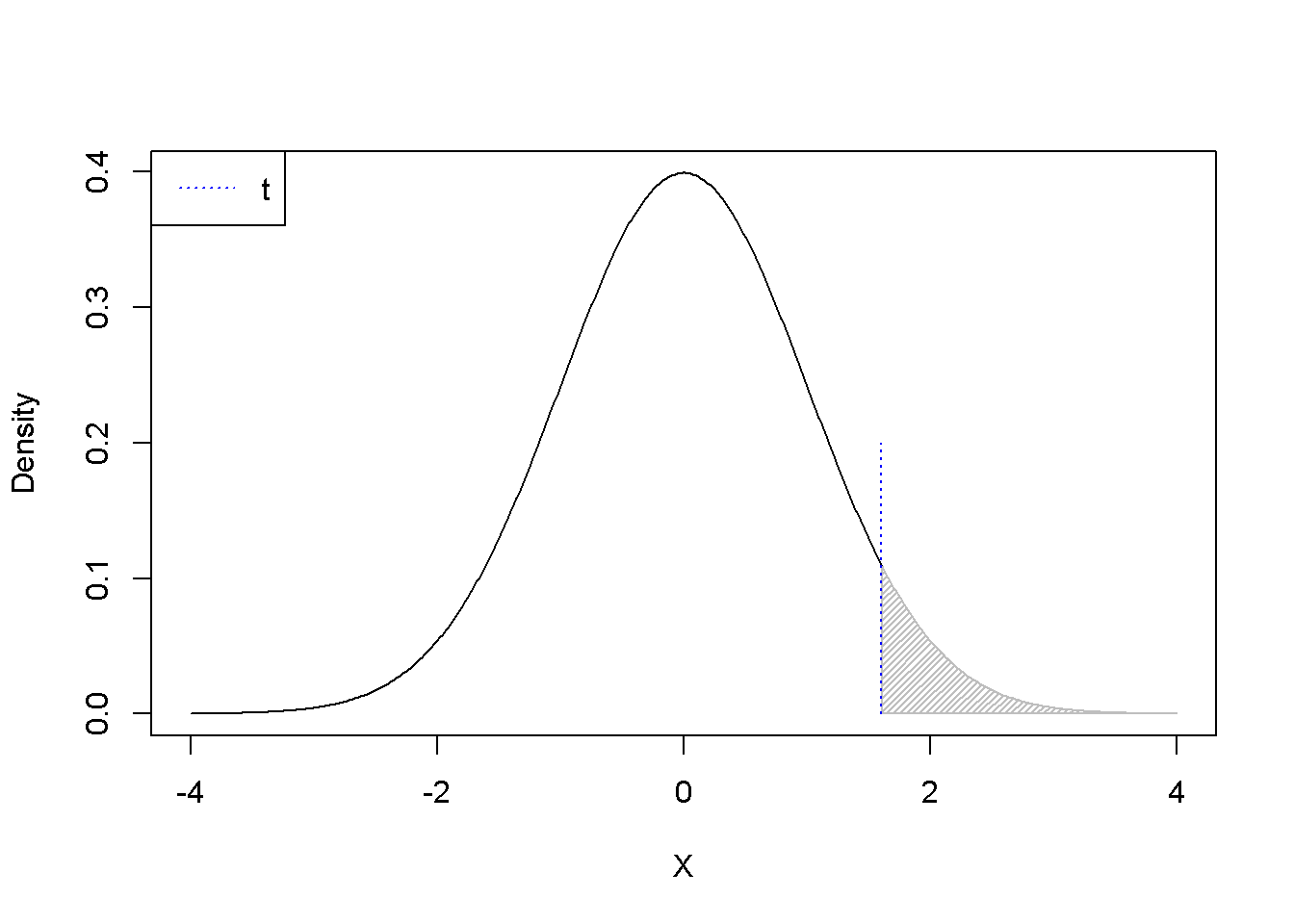
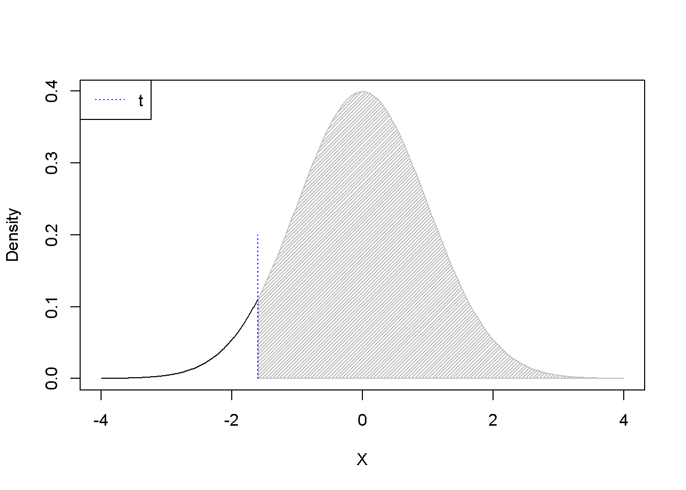
Figure 3.5: \(p-\)Values for positive and negative \(t\) as calculated using the formula \(1-pt(t, df)\)
The next sequence uses the values already calculated before, a hypothesized level of food expenditure \(c\)=$250, and an income of $2000; it tests the two-tail hypothesis in Equation \ref{eq:lineartest31e} first using the “critical \(t\)” method, then using the \(p\)-value method.
c <- 250
alpha <- 0.05
t <- (L-c)/seL  # t < tcr --> Reject Ho.
tcr <- qt(1-alpha/2, df)

# Or, we can calculate the p-value, as follows:
p_value <- 2*(1-pt(abs(t), df)) #p<alpha -> Reject Ho
The results are: \(t=2.65\), \(t_{cr}=2.02\), and \(p=0.0116\). Since \(t>t_{cr}\), we reject the null hypothesis. The same result is given by the \(p\)-value method, where the \(p\)-value is twice the probability area determined by the calculated \(t\).