Chapter 5 The Multiple Regression Model
rm(list=ls())
library(PoEdata)
library(knitr)
library(xtable)
library(printr)
library(effects)
library(car)
library(AER)
library(broom)
This chapter uses a few new packages: effects (Fox et al. 2016), car (Fox and Weisberg 2016), and AER, (Kleiber and Zeileis 2015).
5.1 The General Model
A multiple regression model is very similar to the simple regression model, but includes more independent variables. Thus, the interpretation of a slope parameter has to take into account possible changes in other independent variables: a slope parameter, say \(\beta_{k}\), gives the change in the dependent variable, \(y\), when the independent variable \(x_{k}\) increases by one unit while all the other independent variables remain constant. Equation \ref{eq:multigenform5} gives the general form of a multiple regression model, where \(y\), \(x_{k}\), and \(e\) are \(N \times 1\) vectors, \(N\) is the number of observations in the sample, and \(k=1,...,K\) indicates the \(k\)-th independent variable. The notation used in Equation \ref{eq:multigenform5} implies that the first independent variable, \(x_{1}\), is an \(N \times 1\) vector of \(1\)s. \[\begin{equation} y=\beta_{1}+\beta_{2}x_{2}+...+\beta_{K}x_{K}+e \label{eq:multigenform5} \end{equation}\]The model assumptions remain the same, with the additional requirement that no independent variable is a linear combination of the others.
5.2 Example: Big Andy’s Hamburger Sales
The andy dataset includes variables sales, which is monthly revenue to the company in \(\$1000\)s, price, which is a price index of all products sold by Big Andy’s, and advert, the advertising expenditure in a given month, in \(\$1000\)s. Summary statistics for the andy dataset is shown in Table 5.1. The basic andy model is presented in Equation \ref{eq:basicandymod15}. \[\begin{equation} sales=\beta_{1}+\beta_{2}price+\beta_{3}advert+e \label{eq:basicandymod15} \end{equation}\]# Summary statistics
data(andy)
s=tidy(andy)[,c(1:5,8,9)]
kable(s,caption="Summary statistics for dataset $andy$")| column | n | mean | sd | median | min | max |
|---|---|---|---|---|---|---|
| sales | 75 | 77.3747 | 6.488537 | 76.50 | 62.40 | 91.20 |
| price | 75 | 5.6872 | 0.518432 | 5.69 | 4.83 | 6.49 |
| advert | 75 | 1.8440 | 0.831677 | 1.80 | 0.50 | 3.10 |
# The basic *andy* model
data("andy",package="PoEdata")
mod1 <- lm(sales~price+advert, data=andy)
smod1 <- data.frame(xtable(summary(mod1)))
kable(smod1,
caption="The basic multiple regression model",
col.names=c("coefficient", "Std. Error", "t-value", "p-value"),
align="c", digits=3)| coefficient | Std. Error | t-value | p-value | |
|---|---|---|---|---|
| (Intercept) | 118.914 | 6.352 | 18.722 | 0.000 |
| price | -7.908 | 1.096 | -7.215 | 0.000 |
| advert | 1.863 | 0.683 | 2.726 | 0.008 |
Table 5.2 shows that, for any given (but fixed) value of advertising expenditure, an increase in price by \(\$1\) decreases sales by \(\$7908\). On the other hand, for any given price, sales increase by \(\$1863\) when advertising expenditures increase by \(\$1000\).
effprice <- effect("price", mod1)
plot(effprice)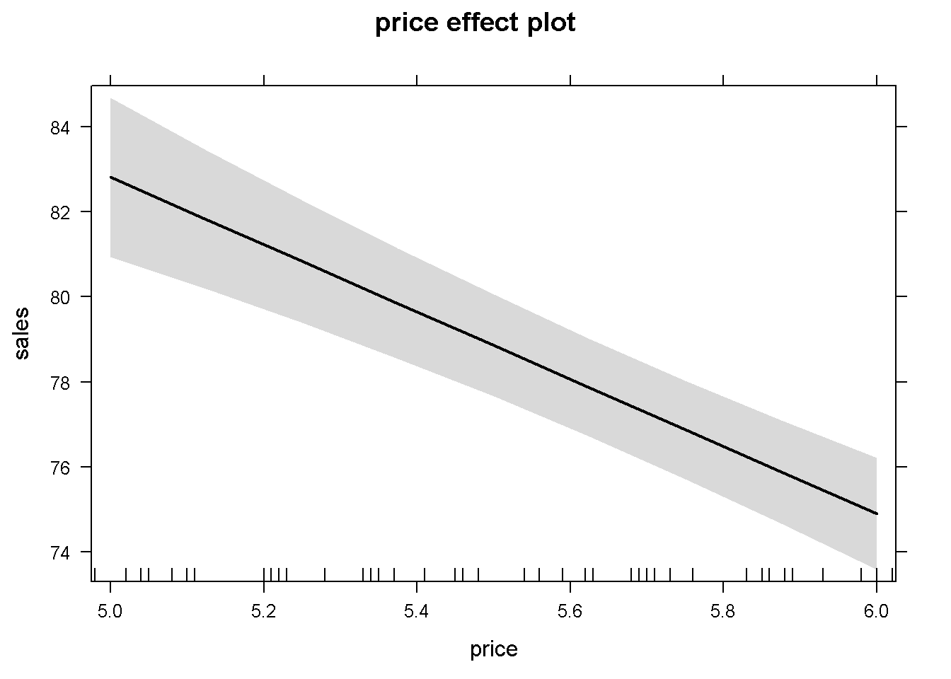
Figure 5.1: The partial effect of \(price\) in the basic \(andy\) regression
summary(effprice)##
## price effect
## price
## 5 5.5 6
## 82.8089 78.8550 74.9011
##
## Lower 95 Percent Confidence Limits
## price
## 5 5.5 6
## 80.9330 77.6582 73.5850
##
## Upper 95 Percent Confidence Limits
## price
## 5 5.5 6
## 84.6849 80.0518 76.2172Figure 5.1 shows the predicted levels of the dependent variable \(sales\) and its 95% confidence band for the sample values of the variable \(price\). In more complex functional forms, the \(R\) function effect() plots the partial effect of a variable for given levels of the other independent variables in the model. The simplest possible call of this function requires, as arguments, the name of the term for which we wish the partial effect (in our example \(price\)), and the object (model) in question. If not otherwise specified, the confidence intervals (band) are determined for a 95% confidence level and the other variables at their means. A simple use of the effects package is presented in Figure 5.2, which plots the partial effects of all variables in the basic \(andy\) model. (Function effect() plots only one graph for one variable, while allEffects() plots all variables in the model.)
alleffandy <- allEffects(mod1)
plot(alleffandy)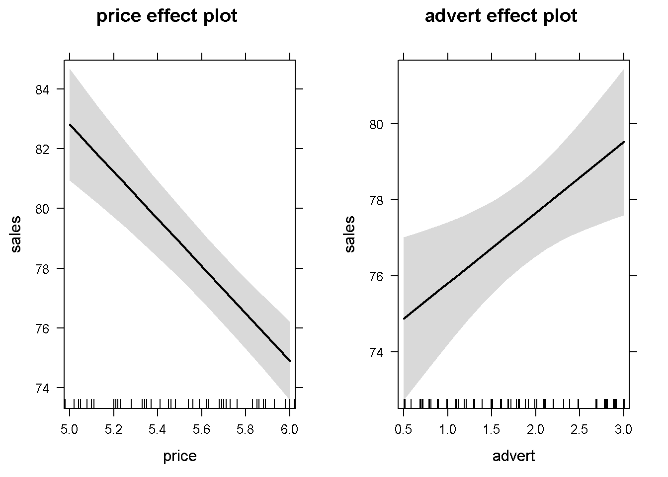
Figure 5.2: Using the function ‘allEffects()’ in the basic \(andy\) model
# Another example of using the function effect()
mod2 <- lm(sales~price+advert+I(advert^2), data=andy)
summary(mod2)
##
## Call:
## lm(formula = sales ~ price + advert + I(advert^2), data = andy)
##
## Residuals:
## Min 1Q Median 3Q Max
## -12.255 -3.143 -0.012 2.851 11.805
##
## Coefficients:
## Estimate Std. Error t value Pr(>|t|)
## (Intercept) 109.719 6.799 16.14 < 2e-16 ***
## price -7.640 1.046 -7.30 3.2e-10 ***
## advert 12.151 3.556 3.42 0.0011 **
## I(advert^2) -2.768 0.941 -2.94 0.0044 **
## ---
## Signif. codes: 0 '***' 0.001 '**' 0.01 '*' 0.05 '.' 0.1 ' ' 1
##
## Residual standard error: 4.65 on 71 degrees of freedom
## Multiple R-squared: 0.508, Adjusted R-squared: 0.487
## F-statistic: 24.5 on 3 and 71 DF, p-value: 5.6e-11plot(effect("I(advert^2)", mod2))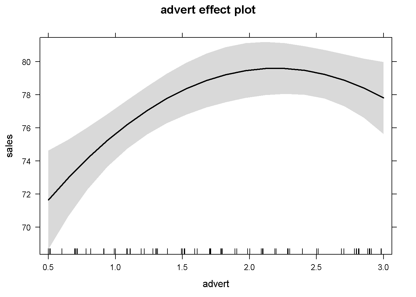
Figure 5.3: An example of using the function ‘effect’ in a quadratic model
Figure 5.3 is an example of using the effect() function to plot the partial effect of a quadratic independent variable. I chose to insert the I(advert^2) term to indicate that the variable of interest needs to be specified exactly as it appears in the model.
All the methods available in \(R\) for simple linear regression models are available for multiple models as well. Thus, to extract the information generated by the lm() function, we use the similar code as before. As we have already learned, the command ?mod1 gives a list with all the information stored in the mod1 object. The next code sequence illustrates how to access various regression output items for the basic \(andy\) equation.
mod1 <- lm(sales~price+advert, data=andy)
smod1 <- summary(mod1)
df <- mod1$df.residual
N <- nobs(mod1)
b1 <- coef(mod1)[[1]] #or
b2 <- coef(mod1)[["price"]]
b3 <- coef(mod1)[["advert"]]
sighat2 <- smod1$sigma^2
anov <- anova(mod1)
SSE <- anov[3,2]
SST <- sum(anov[,2]) #sum of column 2 in anova
SSR <- SST-SSE
kable(data.frame(vcov(mod1)), align='c', digits=3,
      caption="The coefficient covariance matrix",
col.names=c("(Intercept)", "price", "advert"))| (Intercept) | price | advert | |
|---|---|---|---|
| (Intercept) | 40.343 | -6.795 | -0.748 |
| price | -6.795 | 1.201 | -0.020 |
| advert | -0.748 | -0.020 | 0.467 |
The covariance matrix, or the variance-covariance matrix shown in Table 5.3 contains all the estimated variances and covariances of the regression coefficients. These are useful when testing hypotheses about individual coefficients or combinations of those.
5.3 Interval Estimation in Multiple Regression
Interval estimation is similar with the one we have studied in the simple regression model, except the number of degrees of freedom is now \(N-K\), where \(K\) is the number of regression coefficients to be estimated. In the andy example, \(df=72\) and the variances and covariances of the estimates are given in the following code sequence.
varb1 <- vcov(mod1)[1,1]
varb2 <- vcov(mod1)[2,2]
varb3 <- vcov(mod1)[3,3]
covb1b2 <- vcov(mod1)[1,2]
covb1b3 <- vcov(mod1)[1,3]
covb2b3 <- vcov(mod1)[2,3]
seb2 <- sqrt(varb2) #standard error of b2
seb3 <- sqrt(varb3)
With the calculated standard error of \(b_{2}\), \(se(b_{2})=1.096\), we can now determine a \(95\%\) confidence interval, as shown in the following code lines. The code also shows using the \(R\) function confint(model, parm, level) to check our results.
alpha <- 0.05
tcr <- qt(1-alpha/2, df)
lowb2 <- b2-tcr*seb2
upb2 <- b2+tcr*seb2
lowb3 <- b3-tcr*seb3
upb3 <- b3+tcr*seb3
confints <- confint(mod1, parm=c("price", "advert"), level=0.95)
kable(data.frame(confints),
  caption="Confidence intervals for 'price' and 'advert'",
align="c", col.names=c("lowb", "upb"), digits=4)| lowb | upb | |
|---|---|---|
| price | -10.0927 | -5.7230 |
| advert | 0.5007 | 3.2245 |
Finding an interval estimate for a linear combination of the parameters is often needed. Suppose one is interested in determining an interval estimate for sales when the price decreases by \(40\) cents and the advertising expenditure increases by \(\$800\) (see Equation \ref{eq:linearconfintandy5}) in the andy basic equation.
\[\begin{equation} \lambda=0\beta_{1} -0.4\beta_{2} +0.8\beta_{3} \label{eq:linearconfintandy5} \end{equation}\]alpha <- 0.1
tcr <- qt(1-alpha/2, df)
a1 <- 0
a2 <- -0.4
a3 <- 0.8
L <- a1*b1+a2*b2+a3*b3
varL <- a1^2*varb1+a2^2*varb2+a3^2*varb3+
2*a1*a2*covb1b2+2*a1*a3*covb1b3+2*a2*a3*covb2b3
seL <- sqrt(varL)
lowbL <- L-tcr*seL
upbL <- L+tcr*seLThe calculated confidence interval is \((3.471 , 5.836)\). Let us calculate the variance of a linear combination of regression parameters in a more general way to take advantage of \(R\)’s excellent capabilities of working with complex data structures such as lists, vectors, and matrices. This code sequence introduces a few new elements, such as matrix transposition and multiplication, as well as turning a list into a vector. The matrix multiplication operator in \(R\) is %*% and the transposition operator is t().
a <- c(0, -0.4, 0.8) # vector
b <- as.numeric(coef(mod1))# vector of coefficients
L <- L <- sum(a*b) # sum of elementwise products
V <- vcov(mod1) # the variance-covariance matrix
A <- as.vector(a) # (indeed not necessary)
varL <- as.numeric(t(A) %*% V %*% A)
5.4 Hypothesis Testing in Multiple Regression
The process of testing hypotheses about a single parameter is similar to the one we’ve seen in simple regression, the only difference consisting in the number of degrees of freedom. As an example, let us test the significance of \(\beta_{2}\) of the basic andy equation. The hypotheses are given in Equation \ref{eq:signiftestandy5}.
\[\begin{equation} H_{0}: \beta_{2}=0, \;\;\; H_{A}: \beta_{2}\neq 0 \label{eq:signiftestandy5} \end{equation}\]alpha <- 0.05
df <- mod1$df.residual
tcr <- qt(1-alpha/2, df)
b2 <- coef(mod1)[["price"]]
seb2 <- sqrt(vcov(mod1)[2,2])
t <- b2/seb2The calculated \(t\) is equal to \(-7.215\), which is less than \(-t_{cr}=-1.993\), indicating that the null hypothesis is rejected and that \(\beta_{2}\) is significantly different from zero. As usual, we can perform the same test using the \(p\)-value instead of \(t_{cr}\).
t <- b2/seb2
pval <- 2*(1-pt(abs(t), df)) #two-tail test
The calculated \(p\)-value is \(4.423999\times 10^{-10}\). Since this is less than \(\alpha\) we reject, again, the null hypothesis \(H_{0}:\beta_{2}=0\). Let us do the same for \(\beta_{3}\):
alpha <- 0.05
df <- mod1$df.residual
tcr <- qt(1-alpha/2, df)
b3 <- coef(mod1)[[3]]
seb3 <- sqrt(vcov(mod1)[3,3])
tval <- b3/seb3
Calculated \(t=2.726\), and \(t_{cr}=1.993\). Since \(t>t_{cr}\) we reject the null hypothesis and conclude that there is a statistically significant relationship between \(advert\) and \(sales\). The same result can be obtained using the \(p\)-value method:
pval <- 2*(1-pt(abs(tval), df))Result: \(p\)-value \(=0.008038 < \alpha\). \(R\) shows the two-tail \(t\) and \(p\) values for coefficients in regression output (see Table 5.2).
A one-tail hypothesis testing can give us information about price elasitcity of demand in the basic andy equation in Table 5.2. Let us test the hypothesis described in Equation \ref{eq:onetailb2andy5} at a \(5\%\) significance level. The calculated value of \(t\) is the same, but \(t_{cr}\) corresponds now not to \(\frac{\alpha}{2}\) but to \(\alpha\). \[\begin{equation} H_{0}:\beta_{2}\ge 0,\;\;\; H_{A}:\beta_{2}<0 \label{eq:onetailb2andy5} \end{equation}\]alpha <- 0.05
tval <- b2/seb2
tcr <- -qt(1-alpha, df) #left-tail test
pval <- pt(tval, df)The results \(t=-7.215\), \(t_{cr}=-1.666\) show that the calculated \(t\) falls in the (left-tail) rejection region. The \(p\)-value, which is equal to \(2.211999\times 10^{-10}\), is less than \(\alpha\), also rejects the null hypothesis.
Here is how the \(p\)-values should be calculated, depending on the type of test:
- Two-tail test (\(H_{A}: \beta_{2}\neq 0\)),
p-value <- 2*(1-pt(abs(t), df)) - Left-tail test (\(H_{A}: \beta_{2}< 0\)),
p-value <- pt(t, df) - Right-tail test (\(H_{A}: \beta_{2}> 0\)),
p-value <- 1-pt(t, df)
tval <- (b3-1)/seb3
pval <- 1-pt(tval,df)
The calculated \(p\)-value is \(0.105408\), which is greater than \(\alpha\), showing that we cannot reject the null hypothesis \(H_{0}:\beta_{3}\le 1\) at \(\alpha =0.05\). In other words, increasing advertising expenditure by \(\$1\) may or may not increase sales by more than \(\$1\).
Testing hypotheses for linear combinations of coefficients resambles the interval estimation procedure. Suppose we wish to determine if lowering the price by \(20\) cents increases sales more than would an increase in advertising expenditure by \(\$500\). The hypothesis to test this conjecture is given in Equation \ref{eq:linearhypandy5}. \[\begin{equation} H_{0}:0\beta_{1}-0.2\beta_{2}-0.5\beta_{3}\le 0, \;\;\; H_{A}:0\beta_{1}-0.2\beta_{2}-0.5\beta_{3}> 0 \label{eq:linearhypandy5} \end{equation}\]Let us practice the matrix form of testing this hypotesis. \(R\) functions having names that start with as. coerce a certain structure into another, such as a named list into a vector (names are removed and only numbers remain).
A <- as.vector(c(0, -0.2, -0.5))
V <- vcov(mod1)
L <- as.numeric(t(A) %*% coef(mod1))
seL <- as.numeric(sqrt(t(A) %*% V %*% A))
tval <- L/seL
pval <- 1-pt(tval, df) # the result (p-value)
The answer is \(p\)-value= \(0.054619\), which barely fails to reject the null hypothesis. Thus, the conjecture that a decrease in price by \(20\) cents is more effective than an increase in advertising by \(\$800\) is not supported by the data.
For two-tail linear hypotheses, \(R\) has a built-in function, linearHypothesis(model, hypothesis), in the package car. This function tests hypotheses based not on \(t\)-statistics as we have done so far, but based on an \(F\)-statistic. However, the \(p\)-value criterion to reject or not the null hypothesis is the same: reject if \(p\)-value is less than \(\alpha\). Let us use this function to test the two-tail hypothesis similar to the one given in Equation \ref{eq:linearhypandy5}. (Note that the linearHypothesis() function can test not only one hypothesis, but a set of simultaneous hypotheses.)
hypothesis <- "-0.2*price = 0.5*advert"
test <- linearHypothesis (mod1, hypothesis)
Fstat <- test$F[2]
pval <- 1-pf(Fstat, 1, df)
The calculated \(p\)-value is \(0.109238\), which shows that the null hypothesis cannot be rejected. There are a few new elements, besides the use of the linearHypothesis function in this code sequence. First, the linearHypothesis() function creates an \(R\) object that contains several items, one of which is the \(F\)-statistic we are looking for. This object is shown in Table 5.5 and it is named test in our code. The code element test$F[2] extracts the \(F\)-statistic from the linearHypothesis() object.
Second, please note that the \(F\)-statistic has two ‘degrees of freedom’ parameters, not only one as the \(t\)-statistic does. The first degree of freedom is equal to the number of simultaneous hypotheses to be tested (in our case only one); the second is the number of degrees of freedom in the model, \(df=N-K\).
Last, the function that calculates the \(p\)-value is pf(Fval, df1, df2), where Fval is the calculated value of the \(F\)-statistic, and df1 and df2 are the two degrees of freedom parameters of the \(F\)-statistic.
kable(test, caption="The `linearHypothesis()` object")| Res.Df | RSS | Df | Sum of Sq | F | Pr(>F) |
|---|---|---|---|---|---|
| 73 | 1781.73 | NA | NA | NA | NA |
| 72 | 1718.94 | 1 | 62.7874 | 2.62993 | 0.109238 |
5.5 Polynomial Regression Models
A polynomial multivariate regression model may include several independent variables at various powers. In such models, the partial (or marginal) effect of a regressor \(x_{k}\) on the response \(y\) is determined by the partial derivative \(\frac{\partial y}{\partial x_{k}}\). Let us consider again the basic andy model with the added advert quadratic term as presented in Equation \ref{eq:quadraticAndy5}. \[\begin{equation} sales_{i}=\beta_{1}+\beta_{2}price_{i}+\beta_{3}advert_{i}+\beta_{4}advert_{i}^2+e_{i} \label{eq:quadraticAndy5} \end{equation}\]As we have noticed before, the quadratic term is introduced into the model using the function I() to indicate the presence of a mathematical operator. Table 5.6 presents a summary of the regression output from the model described in Equation \ref{eq:quadraticAndy5}.
mod2 <- lm(sales~price+advert+I(advert^2),data=andy)
smod2 <- summary(mod2)
tabl <- data.frame(xtable(smod2))
names(tabl) <- c("Estimate",
                 "Std. Error", "t", "p-Value")
kable(tabl, digits=3, align='c',
caption="The quadratic version of the $andy$ model")| Estimate | Std. Error | t | p-Value | |
|---|---|---|---|---|
| (Intercept) | 109.719 | 6.799 | 16.137 | 0.000 |
| price | -7.640 | 1.046 | -7.304 | 0.000 |
| advert | 12.151 | 3.556 | 3.417 | 0.001 |
| I(advert^2) | -2.768 | 0.941 | -2.943 | 0.004 |
advlevels <- c(0.5, 2)
b3 <- coef(mod2)[[3]]
b4 <- coef(mod2)[[4]]
DsDa <- b3+b4*advlevels
The calculated marginal effects for the two levels of advertising expenditure are, respectively, \(10.767254\) and \(6.615309\), which shows, as expected, diminishing returns to advertising at any given price.
Often, marginal effects or other quantities are non-linear functions of the parameters of a regression model. The delta method allows calculating the variance of such quantities using a Taylor series approximation. This method is, howver, valid only in a vicinity of a point, as any mathematical object involving derivatives.
Suppose we wish to test a hypothesis such as the one in Equation \ref{eq:deltagfunction5}, where \(c\) is a constant. \[\begin{equation} H_{0}: g(\beta_{1},\beta_{2})=c \label{eq:deltagfunction5} \end{equation}\] The delta method consists in estimating the variance of the function \(g(\beta_{1},\beta_{2})\) around some given data point, using the formula in Equation \ref{eq:deltavargen5}, where \(g_{i}\) stands for \(\frac{\partial g}{\partial \beta_{i}}\) calculated at the point \(\beta=b\). \[\begin{equation} var(g)=g_{1}^2var(b_{1})+g_{2}^2var(b_{2})+2g_{1}g_{2}cov(b_{1},b_{2}) \label{eq:deltavargen5} \end{equation}\] Let us apply this method to find a confidence interval for the optimal level of advertising in the andy quadratic equation, \(g\), which is given by Equation \ref{eq:optimaladvertAndy}. \[\begin{equation} \hat g=\frac{1-b_{3}}{2b_{4}} \label{eq:optimaladvertAndy} \end{equation}\] Equation \ref{eq:optimaladvderivatives} shows the derivatives of function \(g\). \[\begin{equation} \hat g_{3}=-\frac{1}{2b_{4}}, \;\;\; \hat g_{4} = -\frac{1-b_{3}}{2b_{4}^2}. \label{eq:optimaladvderivatives} \end{equation}\]alpha <- 0.05
df <- mod2$df.residual
tcr <- qt(1-alpha/2, df)
g <- (1-b3)/(2*b4)
g3 <- -1/(2*b4)
g4 <- -(1-b3)/(2*b4^2)
varb3 <- vcov(mod2)[3,3]
varb4 <- vcov(mod2)[4,4]
covb3b4 <- vcov(mod2)[3,4]
varg <- g3^2*varb3+g4^2*varb4+2*g3*g4*covb3b4
seg <- sqrt(varg)
lowbg <- g-tcr*seg
upbg <- g+tcr*segThe point estimate of the optimal advertising level is \(2.014\), with its confidence interval (\(1.758\), \(2.271\)).
5.6 Interaction Terms in Linear Regression
Interaction terms in a regression model combine two or more variables and model interdependences among the variables. In such models, the slope of one variable may depend on another variable. Partial effects are calculated as partial derivatives, similar to the polynomial equations we have already studied, considering the interaction term a a product of the variables involved.
The data file pizza4 includes 40 observations on an individual’s age and his or her spending on pizza. It is natural to believe that there is some connection between a person’s age and her pizza purchases, but also that this effect may depend on the person’s income. Equation \ref{eq:incomeagepizza5} combines \(age\) and \(income\) in an interaction term, while Equation \ref{eq:marginalpizzaage5} shows the marginal effect of \(age\) on the expected pizza purchases.
\[\begin{equation} pizza=\beta_{1}+\beta_{2}age+\beta_{3}income+\beta_{4}(age \times income)+e \label{eq:incomeagepizza5} \end{equation}\] \[\begin{equation} \frac{\widehat{\partial pizza}}{\partial age}=b_{2}+b_{4}income \label{eq:marginalpizzaage5} \end{equation}\]Let us calculate the marginal effect of \(age\) on \(pizza\) for two levels of income, \(\$25\,000\) and \(\$90\,000\). There are two ways to introduce interaction terms in \(R\); first, with a : (colon) symbol, when only the interaction term is created; second, with the * (star) symbol when all the terms involving the variables in the interaction term should be present in the regression. For instance, the code \(x*z\) creates three terms: \(x\), \(z\), and \(x:z\) (this last one is \(x\) ‘interacted’ with \(z\), which is a peculiarity of the \(R\) system).
data("pizza4",package="PoEdata")
mod3 <- lm(pizza~age*income, data=pizza4)
summary(mod3)
##
## Call:
## lm(formula = pizza ~ age * income, data = pizza4)
##
## Residuals:
## Min 1Q Median 3Q Max
## -200.9 -83.8 20.7 85.0 254.2
##
## Coefficients:
## Estimate Std. Error t value Pr(>|t|)
## (Intercept) 161.4654 120.6634 1.34 0.189
## age -2.9774 3.3521 -0.89 0.380
## income 6.9799 2.8228 2.47 0.018 *
## age:income -0.1232 0.0667 -1.85 0.073 .
## ---
## Signif. codes: 0 '***' 0.001 '**' 0.01 '*' 0.05 '.' 0.1 ' ' 1
##
## Residual standard error: 127 on 36 degrees of freedom
## Multiple R-squared: 0.387, Adjusted R-squared: 0.336
## F-statistic: 7.59 on 3 and 36 DF, p-value: 0.000468inc <- c(25, 90)
b2 <- coef(mod3)[[2]]
b4 <- coef(mod3)[[4]]
(DpDa <- b2+b4*inc)## [1] -6.05841 -14.06896The marginal effect of \(age\) is a reduction in pizza expenditure by \(\$6.058407\) for an income of \(\$25\,000\) and by \(\$14.068965\) for an income of \(\$90\,000\).
Equation \ref{eq:wageeqinteractquadr5} is another example of a model involving an interaction term: the wage equation. The equation involves, besides the interaction term, logs of the response (dependent) variable is in logs and a quadratic term. \[\begin{equation} log(wage)=\beta_{1}+\beta_{2}educ+\beta_{3}exper+\beta_{4}(educ\times exper)+\beta_{5}exper^2 + e \label{eq:wageeqinteractquadr5} \end{equation}\] The marginal effect of an extra year of experience is determined, again, by the partial derivative of \(log(wage)\) with respect to \(exper\), as Equation \ref{eq:wageeqpartialeffect5} shows. Here, however, the marginal effect is easier expressed in percentage change, rather than in units of \(wage\). \[\begin{equation} \% \Delta wage\cong 100\,(\beta_{3}+\beta_{4}educ+2\beta_{5}exper)\Delta exper \label{eq:wageeqpartialeffect5} \end{equation}\]Please note that the marginal effect of \(exper\) depends on both education and experience. Let us calculate this marginal effect for the average values of \(educ\) and \(exper\).
data(cps4_small)
meduc <- mean(cps4_small$educ)
mexper <- mean(cps4_small$exper)
mod4 <- lm(log(wage)~educ*exper+I(exper^2), data=cps4_small)
smod4 <- data.frame(xtable(summary(mod4)))
b3 <- coef(mod4)[[3]]
b4 <- coef(mod4)[[4]]
b5 <- coef(mod4)[[5]]
pDwDex <- 100*(b3+b4*meduc+2*b5*mexper)
The result of this calculation is \(\% \Delta wage =-1.698\), which has, apparently, the wrong sign. What could be the cause? Let us look at a summary of the regression output and identify the terms (see Table 5.7).
kable(smod4, caption="Wage equation with interaction and quadratic terms")| Estimate | Std..Error | t.value | Pr…t.. | |
|---|---|---|---|---|
| (Intercept) | 0.529677 | 0.226741 | 2.33604 | 0.019687 |
| educ | 0.127195 | 0.014719 | 8.64167 | 0.000000 |
| exper | 0.062981 | 0.009536 | 6.60447 | 0.000000 |
| I(exper^2) | -0.000714 | 0.000088 | -8.10911 | 0.000000 |
| educ:exper | -0.001322 | 0.000495 | -2.67222 | 0.007658 |
The output table shows that the order of the terms in the regression equation is not the same as in Equation \ref{eq:wageeqinteractquadr5}, which is the effect of using the compact term \(educ*exper\) in the \(R\) code. This places the proper interaction term, \(educ:exper\) in the last position of all terms containing any of the variables involved in the combined term \(educ*exper\). There are a few ways to solve this issue. One is to write the equation code in full, without the shortcut \(educ*exper\); another is to use the names of the terms when retrieving the coefficients, such as b4 <- coef(mod1)[["I(exper^2)"]]; another to change the position of the terms in Equation \ref{eq:wageeqinteractquadr5} according to Table 5.7 and re-calculate the derivative in Equation \ref{eq:wageeqpartialeffect5}. I am going to use the names of the variables, as they appear in Table 5.7, but I also change the names of the parameters to avoid confusion.
bexper <- coef(mod4)[["exper"]]
bint <- coef(mod4)[["educ:exper"]]
bsqr <- coef(mod4)[["I(exper^2)"]]
pDwDex <- 100*(bexper+bint*meduc+2*bsqr*mexper)
The new result indicates that the expected wage increases by \(0.68829\) percent when experience increases by one year, which, at least, has the “right” sign.
5.7 Goodness-of-Fit in Multiple Regression
The coefficient of determination, \(R^2\), has the same formula (Equation \ref{eq:rsquaredmultiplereg5})and interpretation as in the case of the simple regression model. \[\begin{equation} R^2=\frac{SSR}{SST}=1-\frac{SSE}{SST} \label{eq:rsquaredmultiplereg5} \end{equation}\]As we have already seen, the \(R\) function anova() provides a decomposition of the total sum of squares, showing by how much each predictor contributes to the reduction in the residual sum of squares. Let us look at the basic andy model described in Equation \ref{eq:basicandymod15}.
mod1 <- lm(sales~price+advert, data=andy)
smod1 <- summary(mod1)
Rsq <- smod1$r.squared
anov <- anova(mod1)
dfr <- data.frame(anov)
kable(dfr, caption="Anova table for the basic *andy* model")| Df | Sum.Sq | Mean.Sq | F.value | Pr..F. | |
|---|---|---|---|---|---|
| price | 1 | 1219.091 | 1219.0910 | 51.06310 | 0.000000 |
| advert | 1 | 177.448 | 177.4479 | 7.43262 | 0.008038 |
| Residuals | 72 | 1718.943 | 23.8742 | NA | NA |
Table 5.8 shows that \(price\) has the largest contribution to the reduction of variablity in the residuals; since total sum of squares is \(SST = 3115.482\) (equal to the sum of column Sum.Sq in Table 5.8), the portion explained by \(price\) is \(1219.091\), the one explained by \(advert\) is \(177.448\), and the portion still remaining in the residuals is \(SSE=1718.943\). The portion of variability explained by regression is equal to the sum of the first two items in the Sum.Sq column of the anova table, those corresponding to \(price\) and \(advert\): \(SSR=1396.539\).
RStudio displays the values of all named variables in the Environment window (the NE panel of your screen). Please check, for instance, that \(R^2\) (named Rsq in the previous code sequence) is equal to \(0.448\).
References
Fox, John, Sanford Weisberg, Michael Friendly, and Jangman Hong. 2016. Effects: Effect Displays for Linear, Generalized Linear, and Other Models. https://CRAN.R-project.org/package=effects.
Fox, John, and Sanford Weisberg. 2016. Car: Companion to Applied Regression. https://CRAN.R-project.org/package=car.
Kleiber, Christian, and Achim Zeileis. 2015. AER: Applied Econometrics with R. https://CRAN.R-project.org/package=AER.