Chapter 8 Heteroskedasticity
rm(list=ls()) #Removes all items in Environment!
library(lmtest) #for coeftest() and bptest().
library(broom) #for glance() and tidy()
library(PoEdata) #for PoE4 datasets
library(car) #for hccm() robust standard errors
library(sandwich)
library(knitr)
library(stargazer)
Reference for the package sandwich (Lumley and Zeileis 2015).
One of the assumptions of the Gauss-Markov theorem is homoskedasticity, which requires that all observations of the response (dependent) variable come from distributions with the same variance \(\sigma^2\). In many economic applications, however, the spread of \(y\) tends to depend on one or more of the regressors \(x\). For example, in the food simple regression model (Equation \ref{eq:foodagain8}) expenditure on food stays closer to its mean (regression line) at lower incomes and to be more spread about its mean at higher incomes. Think just that people have more choices at higher income whether to spend their extra income on food or something else.
\[\begin{equation} food\_exp_{i}=\beta_{1}+\beta_{2}income_{i}+e_{i} \label{eq:foodagain8} \end{equation}\]In the presence of heteroskedasticity, the coefficient estimators are still unbiased, but their variance is incorrectly calculated by the usual OLS method, which makes confidence intervals and hypothesis testing incorrect as well. Thus, new methods need to be applied to correct the variances.
8.1 Spotting Heteroskedasticity in Scatter Plots
When the variance of \(y\), or of \(e\), which is the same thing, is not constant, we say that the response or the residuals are heteroskedastic. Figure 8.1 shows, again, a scatter diagram of the food dataset with the regression line to show how the observations tend to be more spread at higher income.
data("food",package="PoEdata")
mod1 <- lm(food_exp~income, data=food)
plot(food$income,food$food_exp, type="p",
     xlab="income", ylab="food expenditure")
abline(mod1)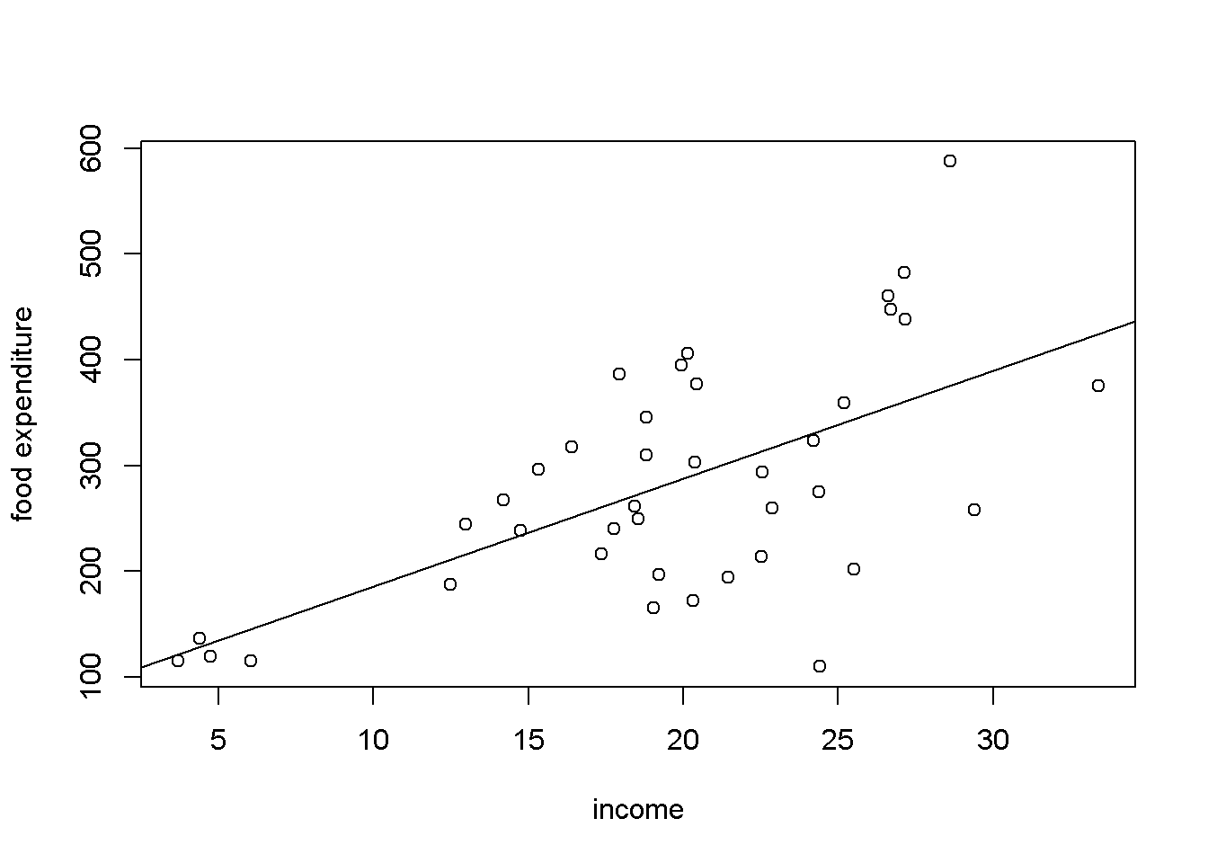
Figure 8.1: Heteroskedasticity in the ‘food’ data
Another useful method to visualize possible heteroskedasticity is to plot the residuals against the regressors suspected of creating heteroskedasticity, or, more generally, against the fitted values of the regression. Figure 8.2 shows both these options for the simple food_exp model.
res <- residuals(mod1)
yhat <- fitted(mod1)
plot(food$income,res, xlab="income", ylab="residuals")
plot(yhat,res, xlab="fitted values", ylab="residuals")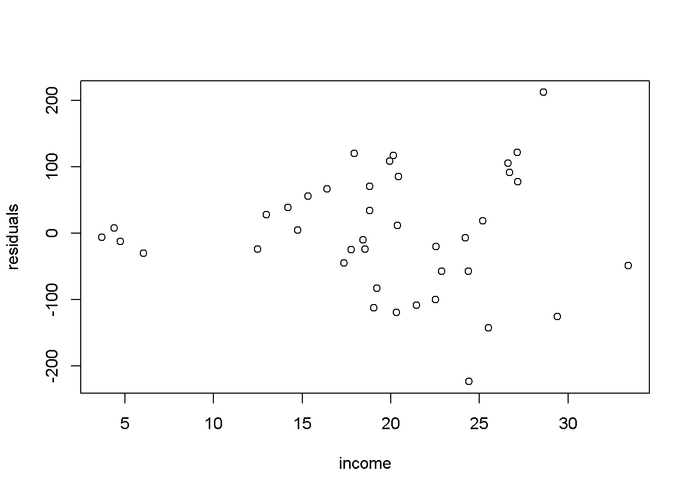
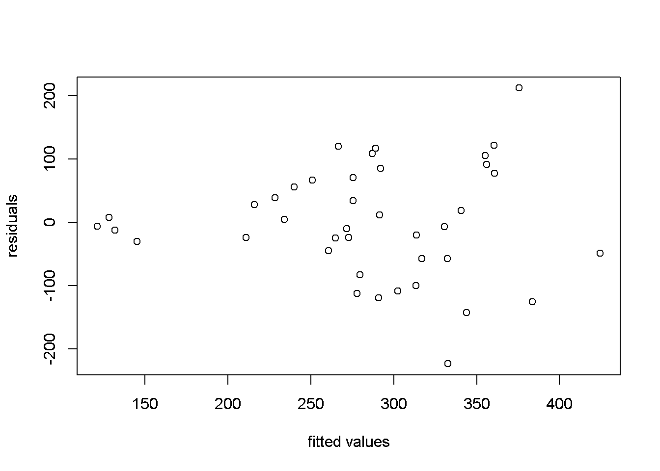
Figure 8.2: Residual plots in the ‘food’ model
8.2 Heteroskedasticity Tests
Suppose the regression model we want to test for heteroskedasticity is the one in Equation \ref{eq:multireggen8}. \[\begin{equation} y_{i}=\beta_{1}+\beta_{2}x_{i2}+...+\beta_{K}x_{iK}+ e_{i} \label{eq:multireggen8} \end{equation}\]The test we are construction assumes that the variance of the errors is a function \(h\) of a number of regressors \(z_{s}\), which may or may not be present in the initial regression model that we want to test. Equation \ref{eq:hetfctn8} shows the general form of the variance function.
\[\begin{equation} var(y_{i})=E(e_{i}^2)=h(\alpha_{1}+\alpha_{2}z_{i2}+...+\alpha_{S}z_{iS}) \label{eq:hetfctn8} \end{equation}\] The variance \(var(y_{i})\) is constant only if all the coefficients of the regressors \(z\) in Equation \ref{eq:hetfctn8} are zero, which provides the null hypothesis of our heteroskedasticity test shown in Equation \ref{eq:hetHo8}. \[\begin{equation} H_{0}: \alpha_{2}=\alpha_{3}=\,...\,\alpha_{S}=0 \label{eq:hetHo8} \end{equation}\] Since we do not know the true variances of the response variable \(y_{i}\), all we can do is to estimate the residuals from the initial model in Equation \ref{eq:multireggen8} and replace \(e_{i}^2\) in Equation \ref{eq:hetfctn8} with the estimated residuals. For a linear function \(h()\), the test equation is, finally, Equation \ref{eq:hetres8}. \[\begin{equation} \hat{e}_{i}^2=\alpha_{1}+\alpha_{2}z_{i2}+...+\alpha_{S}z_{iS}+\nu_{i} \label{eq:hetres8} \end{equation}\]Te relevant test statistic is \(\chi ^2\), given by Equation \ref{eq:chisq8}, where \(R^2\) is the one resulted from Equation \ref{eq:hetres8}.
\[\begin{equation} \chi ^2=N\times R^2 \sim \chi ^{2}_{(S-1)} \label{eq:chisq8} \end{equation}\]The Breusch-Pagan heteroskedasticiy test uses the method we have just described, where the regressors \(z_{s}\) are the variables \(x_{k}\) in the initial model. Let us apply this test to the food model. The function to determine a critical value of the \(\chi ^2\) distribution for a significance level \(\alpha\) and \(S-1\) degrees of freedom is qchisq(1-alpha, S-1).
alpha <- 0.05
mod1 <- lm(food_exp~income, data=food)
ressq <- resid(mod1)^2
#The test equation:
modres <- lm(ressq~income, data=food)
N <- nobs(modres)
gmodres <- glance(modres)
S <- gmodres$df #Number of Betas in model
#Chi-square is always a right-tail test
chisqcr <- qchisq(1-alpha, S-1)
Rsqres <- gmodres$r.squared
chisq <- N*Rsqres
pval <- 1-pchisq(chisq,S-1)
Our test yields a value of the test statistic \(\chi ^2\) of \(7.38\), which is to be compared to the critical \(\chi^{2}_{cr}\) having \(S-1=1\) degrees of freedom and \(\alpha = 0.05\). This critical value is \(\chi ^{2}_{cr}=3.84\). Since the calculated \(\chi ^2\) exceeds the critical value, we reject the null hypothesis of homoskedasticity, which means there is heteroskedasticity in our data and model. Alternatively, we can find the \(p\)-value corresponding to the calculated \(\chi^{2}\), \(p=0.007\).
Let us now do the same test, but using a White version of the residuals equation, in its quadratic form.
modres <- lm(ressq~income+I(income^2), data=food)
gmodres <- glance(modres)
Rsq <- gmodres$r.squared
S <- gmodres$df #Number of Betas in model
chisq <- N*Rsq
pval <- 1-pchisq(chisq, S-1)
The calculated \(p\)-value in this version is \(p=0.023\), which also implies rejection of the null hypothesis of homoskedasticity.
The function bptest() in package lmtest does (the robust version of) the Breusch-Pagan test in \(R\). The following code applies this function to the basic food equation, showing the results in Table 8.1, where ‘statistic’ is the calculated \(\chi^2\).
mod1 <- lm(food_exp~income, data=food)
kable(tidy(bptest(mod1)),
caption="Breusch-Pagan heteroskedasticity test")| statistic | p.value | parameter | method |
|---|---|---|---|
| 7.38442 | 0.006579 | 1 | studentized Breusch-Pagan test |
The test statistic when the null hyppthesis is true, given in Equation \ref{eq:gqf8}, has an \(F\) distribution with its two degrees of freedom equal to the degrees of freedom of the two subsamples, respectively \(N_{1}-K\) and \(N_{0}-K\).
\[\begin{equation} F=\frac{\hat{\sigma}^{2}_{1}}{\hat{\sigma}^{2}_{0}} \label{eq:gqf8} \end{equation}\]Let us apply this test to a \(wage\) equation based on the dataset \(cps2\), where \(metro\) is an indicator variable equal to \(1\) if the individual lives in a metropolitan area and \(0\) for rural area. I will split the dataset in two based on the indicator variable \(metro\) and apply the regression model (Equation \ref{eq:hetwage8}) separately to each group.
\[\begin{equation} wage=\beta_{1}+\beta_{2}educ+\beta_{3}exper+\beta_{4}metro+e \label{eq:hetwage8} \end{equation}\]alpha <- 0.05 #two tail, will take alpha/2
data("cps2", package="PoEdata")
#Create the two groups, m (metro) and r (rural)
m <- cps2[which(cps2$metro==1),]
r <- cps2[which(cps2$metro==0),]
wg1 <- lm(wage~educ+exper, data=m)
wg0 <- lm(wage~educ+exper, data=r)
df1 <- wg1$df.residual #Numerator degrees of freedom
df0 <- wg0$df.residual #Denominatot df
sig1squared <- glance(wg1)$sigma^2
sig0squared <- glance(wg0)$sigma^2
fstat <- sig1squared/sig0squared
Flc <- qf(alpha/2, df1, df0)#Left (lower) critical F
Fuc <- qf(1-alpha/2, df1, df0) #Right (upper) critical FThe results of these calculations are as follows: calculated \(F\) statistic \(F=2.09\), the lower tail critical value \(F_{lc}=0.81\), and the upper tail critical value \(F_{uc}=1.26\). Since the calculated amount is greater than the upper critical value, we reject the hypothesis that the two variances are equal, facing, thus, a heteroskedasticity problem. If one expects the variance in the metropolitan area to be higher and wants to test the (alternative) hypothesis \(H_{0}:\sigma^{2}_{1}\leq \sigma^{2}_{0},\;\;\;\; H_{A}:\sigma^{2}_{1}>\sigma^{2}_{0}\), one needs to re-calcuate the critical value for \(\alpha=0.05\) as follows:
Fc <- qf(1-alpha, df1, df0) #Right-tail testThe critical value for the right tail test is \(F_{c}=1.22\), which still implies rejecting the null hypothesis.
The Goldfeld-Quant test can be used even when there is no indicator variable in the model or in the dataset. One can split the dataset in two using an arbitrary rule. Let us apply the method to the basic \(food\) equation, with the data split in low-income (\(li\)) and high-income (\(hi\)) halves. The cutoff point is, in this case, the median income, and the hypothesis to be tested \[H_{0}: \sigma^{2}_{hi}\le \sigma^{2}_{li},\;\;\;\;H_{A}:\sigma^{2}_{hi} > \sigma^{2}_{li}\]
alpha <- 0.05
data("food", package="PoEdata")
medianincome <- median(food$income)
li <- food[which(food$income<=medianincome),]
hi <- food[which(food$income>=medianincome),]
eqli <- lm(food_exp~income, data=li)
eqhi <- lm(food_exp~income, data=hi)
dfli <- eqli$df.residual
dfhi <- eqhi$df.residual
sigsqli <- glance(eqli)$sigma^2
sigsqhi <- glance(eqhi)$sigma^2
fstat <- sigsqhi/sigsqli #The larger var in numerator
Fc <- qf(1-alpha, dfhi, dfli)
pval <- 1-pf(fstat, dfhi, dfli)
The resulting \(F\) statistic in the \(food\) example is \(F=3.61\), which is greater than the critical value \(F_{cr}=2.22\), rejecting the null hypothesis in favour of the alternative hypothesis that variance is higher at higher incomes. The \(p\)-value of the test is \(p=0.0046\).
In the package lmtest, \(R\) has a specialized function to perform Goldfeld-Quandt tests, the function gqtest which takes, among other arguments, the formula describing the model to be tested, a break point specifying how the data should be split (percentage of the number of observations), what is the alternative hypothesis (“greater”, “two.sided”, or “less”), how the data should be ordered (order.by=), and data=. Let us apply gqtest() to the \(food\) example with the same partition as we have just did before.
foodeq <- lm(food_exp~income, data=food)
tst <- gqtest(foodeq, point=0.5, alternative="greater",
       order.by=food$income)
kable(tidy(tst),
caption="R function `gqtest()` with the 'food' equation")| df1 | df2 | statistic | p.value | method |
|---|---|---|---|---|
| 18 | 18 | 3.61476 | 0.004596 | Goldfeld-Quandt test |
Please note that the results from applying gqtest() (Table 8.2 are the same as those we have already calculated.
8.3 Heteroskedasticity-Consistent Standard Errors
Since the presence of heteroskedasticity makes the lest-squares standard errors incorrect, there is a need for another method to calculate them. White robust standard errors is such a method.
The \(R\) function that does this job is hccm(), which is part of the car package and yields a heteroskedasticity-robust coefficient covariance matrix. This matrix can then be used with other functions, such as coeftest() (instead of summary), waldtest() (instead of anova), or linearHypothesis() to perform hypothesis testing. The function hccm() takes several arguments, among which is the model for which we want the robust standard errors and the type of standard errors we wish to calculate. type can be “constant” (the regular homoskedastic errors), “hc0”, “hc1”, “hc2”, “hc3”, or “hc4”; “hc1” is the default type in some statistical software packages. Let us compute robust standard errors for the basic \(food\) equation and compare them with the regular (incorrect) ones.
foodeq <- lm(food_exp~income,data=food)
kable(tidy(foodeq),caption=
"Regular standard errors in the 'food' equation")| term | estimate | std.error | statistic | p.value |
|---|---|---|---|---|
| (Intercept) | 83.4160 | 43.41016 | 1.92158 | 0.062182 |
| income | 10.2096 | 2.09326 | 4.87738 | 0.000019 |
cov1 <- hccm(foodeq, type="hc1") #needs package 'car'
food.HC1 <- coeftest(foodeq, vcov.=cov1)
kable(tidy(food.HC1),caption=
"Robust (HC1) standard errors in the 'food' equation")| term | estimate | std.error | statistic | p.value |
|---|---|---|---|---|
| (Intercept) | 83.4160 | 27.46375 | 3.03731 | 0.004299 |
| income | 10.2096 | 1.80908 | 5.64356 | 0.000002 |
When comparing Tables 8.3 and 8.4, it can be observed that the robust standard errors are smaller and, since the coefficients are the same, the \(t\)-statistics are higher and the \(p\)-values are smaller. Lower \(p\)-values with robust standard errors is, however, the exception rather than the rule.
Next is an example of using robust standard errors when performing a fictitious linear hypothesis test on the basic ‘andy’ model, to test the hypothesis \(H_{0}: \beta_{2}+\beta_{3}=0\)
data("andy", package="PoEdata")
andy.eq <- lm(sales~price+advert, data=andy)
bp <- bptest(andy.eq) #Heteroskedsticity test
b2 <- coef(andy.eq)[["price"]]
b3 <- coef(andy.eq)[["advert"]]
H0 <- "price+advert=0"
kable(tidy(linearHypothesis(andy.eq, H0,
  vcov=hccm(andy.eq, type="hc1"))),
caption="Linear hypothesis with robust standard errors")| res.df | df | statistic | p.value |
|---|---|---|---|
| 73 | NA | NA | NA |
| 72 | 1 | 23.387 | 7e-06 |
kable(tidy(linearHypothesis(andy.eq, H0)),
caption="Linear hypothesis with regular standard errors")| res.df | rss | df | sumsq | statistic | p.value |
|---|---|---|---|---|---|
| 73 | 2254.71 | NA | NA | NA | NA |
| 72 | 1718.94 | 1 | 535.772 | 22.4415 | 0.000011 |
This example demonstrates how to introduce robust standards errors in a linearHypothesis function. It also shows that, when heteroskedasticity is not significant (bptst does not reject the homoskedasticity hypothesis) the robust and regular standard errors (and therefore the \(F\) statistics of the tests) are very similar.
Just for completeness, I should mention that a similar function, with similar uses is the function vcov, which can be found in the package sandwich.
8.4 GLS: Known Form of Variance
Let us consider the regression equation given in Equation \ref{eq:genheteq8}), where the errors are assumed heteroskedastic.
\[\begin{equation} y_{i}=\beta_{1}+\beta_{2}x_{i}+e_{i},\;\;\;var(e_{i})=\sigma_{i} \label{eq:genheteq8} \end{equation}\]Heteroskedasticity implies different variances of the error term for each observation. Ideally, one should be able to estimate the \(N\) variances in order to obtain reliable standard errors, but this is not possible. The second best in the absence of such estimates is an assumption of how variance depends on one or several of the regressors. The estimator obtained when using such an assumption is called a generalized least squares estimator, gls, which may involve a structure of the errors as proposed in Equation \ref{eq:glsvardef8}, which assumes a linear relationship between variance and the regressor \(x_{i}\) with the unknown parameter \(\sigma^2\) as a proportionality factor.
\[\begin{equation} var(e_{i})=\sigma_{i}^2=\sigma ^2 x_{i} \label{eq:glsvardef8} \end{equation}\]One way to circumvent guessing a proportionality factor in Equation \ref{eq:glsvardef8} is to transform the initial model in Equation \ref{eq:genheteq8} such that the error variance in the new model has the structure proposed in Equation \ref{eq:glsvardef8}. This can be achieved if the initial model is divided through by \(\sqrt x_{i}\) and estimate the new model shown in Equation \ref{eq:glsstar8}. If Equation \ref{eq:glsstar8} is correct, then the resulting estimator is BLUE.
\[\begin{equation} y_{i}^{*}=\beta_{1}x_{i1}^{*}+\beta_{2}x_{i2}^{*}+e_{i}^{*} \label{eq:glsstar8} \end{equation}\]In general, if the initial variables are multiplied by quantities that are specific to each observation, the resulting estimator is called a weighted least squares estimator, wls. Unlike the robust standard errors method for heteroskedasticity correction, gls or wls methods change the estimates of regression coefficients.
The function lm() can do wls estimation if the argument weights is provided under the form of a vector of the same size as the other variables in the model. \(R\) takes the square roots of the weights provided to multiply the variables in the regression. Thus, if you wish to multiply the model by \(\frac{1}{\sqrt {x_{i}}}\), the weights should be \(w_{i}=\frac{1}{x_{i}}\).
Let us apply these ideas to re-estimate the \(food\) equation, which we have determined to be affected by heteroskedasticity.
w <- 1/food$income
food.wls <- lm(food_exp~income, weights=w, data=food)
vcvfoodeq <- coeftest(foodeq, vcov.=cov1)
kable(tidy(foodeq),
caption="OLS estimates for the 'food' equation")| term | estimate | std.error | statistic | p.value |
|---|---|---|---|---|
| (Intercept) | 83.4160 | 43.41016 | 1.92158 | 0.062182 |
| income | 10.2096 | 2.09326 | 4.87738 | 0.000019 |
kable(tidy(food.wls),
caption="WLS estimates for the 'food' equation" )| term | estimate | std.error | statistic | p.value |
|---|---|---|---|---|
| (Intercept) | 78.6841 | 23.78872 | 3.30762 | 0.002064 |
| income | 10.4510 | 1.38589 | 7.54100 | 0.000000 |
kable(tidy(vcvfoodeq),caption=
"OLS estimates for the 'food' equation with robust standard errors" )| term | estimate | std.error | statistic | p.value |
|---|---|---|---|---|
| (Intercept) | 83.4160 | 27.46375 | 3.03731 | 0.004299 |
| income | 10.2096 | 1.80908 | 5.64356 | 0.000002 |
Tables 8.7, 8.8, and 8.9 compare ordinary least square model to a weighted least squares model and to OLS with robust standard errors. The WLS model multiplies the variables by \(1 \, / \, \sqrt{income}\), where the weights provided have to be \(w=1\,/\, income\). The effect of introducing the weights is a slightly lower intercept and, more importantly, different standard errors. Please note that the WLS standard errors are closer to the robust (HC1) standard errors than to the OLS ones.
8.5 Grouped Data
We have seen already (Equation \ref{eq:gqnull8}) how a dichotomous indicator variable splits the data in two groups that may have different variances. The generalized least squares method can account for group heteroskedasticity, by choosing appropriate weights for each group; if the variables are transformed by multiplying them by \(1/\sigma_{j}\), for group \(j\), the resulting model is homoskedastic. Since \(\sigma_{j}\) is unknown, we replace it with its estimate \(\hat \sigma_{j}\). This method is named feasible generalized least squares.
data("cps2", package="PoEdata")
rural.lm <- lm(wage~educ+exper, data=cps2, subset=(metro==0))
sigR <- summary(rural.lm)$sigma
metro.lm <- lm(wage~educ+exper, data=cps2, subset=(metro==1))
sigM <- summary(metro.lm)$sigma
cps2$wght <- rep(0, nrow(cps2))
# Create a vector of weights
for (i in 1:1000)
{
  if (cps2$metro[i]==0){cps2$wght[i] <- 1/sigR^2}
  else{cps2$wght[i] <- 1/sigM^2}
}
wge.fgls <- lm(wage~educ+exper+metro, weights=wght, data=cps2)
wge.lm <- lm(wage~educ+exper+metro, data=cps2)
wge.hce <- coeftest(wge.lm, vcov.=hccm(wge.lm, data=cps2))
stargazer(rural.lm, metro.lm, wge.fgls,wge.hce,
  header=FALSE,
  title="OLS vs. FGLS estimates for the 'cps2' data",
  type=.stargazertype, # "html" or "latex" (in index.Rmd)
  keep.stat="n",  # what statistics to print
  omit.table.layout="n",
  star.cutoffs=NA,
  digits=3,
#  single.row=TRUE,
  intercept.bottom=FALSE, #moves the intercept coef to top
  column.labels=c("Rural","Metro","FGLS", "HC1"),
  dep.var.labels.include = FALSE,
  model.numbers = FALSE,
  dep.var.caption="Dependent variable: wage",
  model.names=FALSE,
star.char=NULL) #supresses the stars| Dependent variable: wage | ||||
| Rural | Metro | FGLS | HC1 | |
| Constant | -6.166 | -9.052 | -9.398 | -9.914 |
| (1.899) | (1.189) | (1.020) | (1.218) | |
| educ | 0.956 | 1.282 | 1.196 | 1.234 |
| (0.133) | (0.080) | (0.069) | (0.084) | |
| exper | 0.126 | 0.135 | 0.132 | 0.133 |
| (0.025) | (0.018) | (0.015) | (0.016) | |
| metro | 1.539 | 1.524 | ||
| (0.346) | (0.346) | |||
| Observations | 192 | 808 | 1,000 | |
The table titled “OLS, vs. FGLS estimates for the ‘cps2’ data” helps comparing the coefficients and standard errors of four models: OLS for rural area, OLS for metro area, feasible GLS with the whole dataset but with two types of weights, one for each area, and, finally, OLS with heteroskedasticity-consistent (HC1) standard errors. Please be reminded that the regular OLS standard errors are not to be trusted in the presence of heteroskedasticity.
The previous code sequence needs some explanation. It runs two regression models, rural.lm and metro.lm just to estimate \(\hat \sigma_{R}\) and \(\hat \sigma_{M}\) needed to calculate the weights for each group. The subsets, this time, were selected directly in the lm() function through the argument subset=, which takes as argument some logical expression that may involve one or more variables in the dataset. Then, I create a new vector of a size equal to the number of observations in the dataset, a vector that will be populated over the next few code lines with weights. I choose to create this vector as a new column of the dataset cps2, a column named wght. With this the hard part is done; I just need to run an lm() model with the option weights=wght and that gives my FGLS coefficients and standard errors.
The next lines make a for loop runing through each observation. If observation \(i\) is a rural area observation, it receives a weight equal to \(1/\sigma_{R}^2\); otherwise, it receives the weight \(1/\sigma_{M}^2\). Why did I square those \(sigmas\)? Because, remember, the argument weights in the lm() function requires the square of the factor multiplying the regression model in the WLS method.
The remaining part of the code repeats models we ran before and places them in one table for making comparison easier.
8.6 GLS: Unknown Form of Variance
Suppose we wish to estimate the model in Equation \ref{eq:genericeq8}, where the errors are known to be heteroskedastic but their variance is an unknown function of \(S\) some variables \(z_{s}\) that could be among the regressors in our model or other variables. \[\begin{equation} y_{i}=\beta_{1}+\beta_{2}x_{i2}+...\beta_{k}x_{iK}+e_{i} \label{eq:genericeq8} \end{equation}\]Equation \ref{eq:varfuneq8} uses the residuals from Equation \ref{eq:genericeq8} as estimates of the variances of the error terms and serves at estimating the functional form of the variance. If the assumed functional form of the variance is the exponential function \(var(e_{i})=\sigma_{i}^{2}=\sigma ^2 x_{i}^{\gamma}\), then the regressors \(z_{is}\) in Equation \ref{eq:varfuneq8} are the logs of the initial regressors \(x_{is}\), \(z_{is}=log(x_{is})\).
\[\begin{equation} ln(\hat{e}_{i}^{2})=\alpha_{1}+\alpha_{2}z_{i2}+...+\alpha_{S}z_{iS}+\nu_{i} \label{eq:varfuneq8} \end{equation}\]The variance estimates for each error term in Equation \ref{eq:genericeq8} are the fitted values, \(\hat \sigma_{i}^2\) of Equation \ref{eq:varfuneq8}, which can then be used to construct a vector of weights for the regression model in Equation \ref{eq:genericeq8}. Let us follow these steps on the \(food\) basic equation where we assume that the variance of error term \(i\) is an unknown exponential function of income. So, the purpose of the following code fragment is to determine the weights and to supply them to the lm() function. Remember, lm() multiplies each observation by the square root of the weight you supply. For instance, if you want to multiply the observations by \(1/\sigma_{i}\), you should supply the weight \(w_{i}=1/\sigma_{i}^2\).
data("food", package="PoEdata")
food.ols <- lm(food_exp~income, data=food)
ehatsq <- resid(food.ols)^2
sighatsq.ols  <- lm(log(ehatsq)~log(income), data=food)
vari <- exp(fitted(sighatsq.ols))
food.fgls <- lm(food_exp~income, weights=1/vari, data=food)stargazer(food.ols, food.HC1, food.wls, food.fgls,
header=FALSE,
title="Comparing various 'food' models",
type=.stargazertype, # "html" or "latex" (in index.Rmd)
keep.stat="n", # what statistics to print
omit.table.layout="n",
star.cutoffs=NA,
digits=3,
# single.row=TRUE,
intercept.bottom=FALSE, #moves the intercept coef to top
column.labels=c("OLS","HC1","WLS","FGLS"),
dep.var.labels.include = FALSE,
model.numbers = FALSE,
dep.var.caption="Dependent variable: 'food expenditure'",
model.names=FALSE,
star.char=NULL) #supresses the stars| Dependent variable: ‘food expenditure’ | ||||
| OLS | HC1 | WLS | FGLS | |
| Constant | 83.416 | 83.416 | 78.684 | 76.054 |
| (43.410) | (27.464) | (23.789) | (9.713) | |
| income | 10.210 | 10.210 | 10.451 | 10.633 |
| (2.093) | (1.809) | (1.386) | (0.972) | |
| Observations | 40 | 40 | 40 | |
The table titled “Comparing various ‘food’ models” shows that the FGLS with unknown variances model substantially lowers the standard errors of the coefficients, which in turn increases the \(t\)-ratios (since the point estimates of the coefficients remain about the same), making an important difference for hypothesis testing.
For a few classes of variance functions, the weights in a GLS model can be calculated in \(R\) using the varFunc() and varWeights() functions in the package nlme.
8.7 Heteroskedasticity in the Linear Probability Model
As we have already seen, the linear probability model is, by definition, heteroskedastic, with the variance of the error term given by its binomial distribution parameter \(p\), the probability that \(y\) is equal to 1, \(var(y)=p(1-p)\), where \(p\) is defined in Equation \ref{eq:binomialp8}.
\[\begin{equation} p=\beta_{1}+\beta_{2}x_{2}+...+\beta_{K}x_{K}+e \label{eq:binomialp8} \end{equation}\]Thus, the linear probability model provides a known variance to be used with GLS, taking care that none of the estimated variances is negative. One way to avoid negative or greater than one probabilities is to artificially limit them to the interval \((0,1)\).
Let us revise the \(coke\) model in dataset coke using this structure of the variance.
data("coke", package="PoEdata")
coke.ols <- lm(coke~pratio+disp_coke+disp_pepsi, data=coke)
coke.hc1 <- coeftest(coke.ols, vcov.=hccm(coke.ols, type="hc1"))
p <- fitted(coke.ols)
# Truncate negative or >1 values of p
pt<-p
pt[pt<0.01] <- 0.01
pt[pt>0.99] <- 0.99
sigsq <- pt*(1-pt)
wght <- 1/sigsq
coke.gls.trunc <- lm(coke~pratio+disp_coke+disp_pepsi,
                  data=coke, weights=wght)
# Eliminate negative or >1 values of p
p1 <- p
p1[p1<0.01 | p1>0.99] <- NA
sigsq <- p1*(1-p1)
wght <- 1/sigsq
coke.gls.omit <- lm(coke~pratio+disp_coke+disp_pepsi,
data=coke, weights=wght)stargazer(coke.ols, coke.hc1, coke.gls.trunc, coke.gls.omit,
header=FALSE,
title="Comparing various 'coke' models",
type=.stargazertype, # "html" or "latex" (in index.Rmd)
keep.stat="n", # what statistics to print
omit.table.layout="n",
star.cutoffs=NA,
digits=4,
# single.row=TRUE,
intercept.bottom=FALSE, #moves the intercept coef to top
column.labels=c("OLS","HC1","GLS-trunc","GLS-omit"),
dep.var.labels.include = FALSE,
model.numbers = FALSE,
dep.var.caption="Dependent variable: 'choice of coke'",
model.names=FALSE,
star.char=NULL) #supresses the stars| Dependent variable: ‘choice of coke’ | ||||
| OLS | HC1 | GLS-trunc | GLS-omit | |
| Constant | 0.8902 | 0.8902 | 0.6505 | 0.8795 |
| (0.0655) | (0.0653) | (0.0568) | (0.0594) | |
| pratio | -0.4009 | -0.4009 | -0.1652 | -0.3859 |
| (0.0613) | (0.0604) | (0.0444) | (0.0527) | |
| disp_coke | 0.0772 | 0.0772 | 0.0940 | 0.0760 |
| (0.0344) | (0.0339) | (0.0399) | (0.0353) | |
| disp_pepsi | -0.1657 | -0.1657 | -0.1314 | -0.1587 |
| (0.0356) | (0.0344) | (0.0354) | (0.0360) | |
| Observations | 1,140 | 1,140 | 1,124 | |
References
Lumley, Thomas, and Achim Zeileis. 2015. Sandwich: Robust Covariance Matrix Estimators. https://CRAN.R-project.org/package=sandwich.