Chapter 7 Using Indicator Variables

rm(list=ls())
library(bookdown)
library(PoEdata)#for PoE datasets
library(knitr)  #for referenced tables with kable()
library(xtable) #makes data frame for kable
library(printr) #automatically prints output nicely
library(effects)
library(car)
library(AER)
library(broom) #for tidy lm output and function glance()
library(stats)
library(lmtest)#for coeftest() and other test functions 
library(stargazer) #nice and informative tables

This chapter introduces the package lmtest (Hothorn et al. 2015).

7.1 Factor Variables

Indicator variables show the presence of a certain non-quantifiable attribute, such as whether an individual is male or female, or whether a house has a swimming pool. In $R$ , an indicator variable is called factor, category, or ennumerated type and there is no distinction between binary (such as yes-no, or male-female) or multiple-category factors.

Factors can be either numerical or character variables, ordered or not. $R$ automatically creates dummy variables for each category within a factor variable and excludes a (baseline) category from a model. The choice of the baseline category, as well as which categories should be included can be changed using the function contrasts().

The following code fragment loads the utown data, declares the indicator variables utown, pool, and fplace as factors, and displays a summary statistics table (Table 7.1). Please notice that the factor variables are represented in the summary table as count data, i.e., how many observations are in each category.

library(stargazer); library(ggplot2)
data("utown", package="PoEdata")
utown$utown <- as.factor(utown$utown)
utown$pool <- as.factor(utown$pool)
utown$fplace <- as.factor(utown$fplace)
kable(summary.data.frame(utown), 
          caption="Summary for 'utown' dataset")

Table 7.1: Summary for ‘utown’ dataset
price	sqft	age	utown	pool	fplace
Min. :134	Min. :20.0	Min. : 0.00	0:481	0:796	0:482
1st Qu.:216	1st Qu.:22.8	1st Qu.: 3.00	1:519	1:204	1:518
Median :246	Median :25.4	Median : 6.00	NA	NA	NA
Mean :248	Mean :25.2	Mean : 9.39	NA	NA	NA
3rd Qu.:278	3rd Qu.:27.8	3rd Qu.:13.00	NA	NA	NA
Max. :345	Max. :30.0	Max. :60.00	NA	NA	NA

This example uses the utown dataset, where prices are in thousands, sqft is the living area is hundreds of square feet, and utown marks houses located near university.

7.2 Examples

mod4 <- lm(price~utown*sqft+age+pool+fplace, data=utown)
kable(tidy(mod4), caption="The 'house prices' model")

Table 7.2: The ‘house prices’ model
term	estimate	std.error	statistic	p.value
(Intercept)	24.499985	6.191721	3.95689	0.000081
utown1	27.452952	8.422582	3.25945	0.001154
sqft	7.612177	0.245176	31.04775	0.000000
age	-0.190086	0.051205	-3.71229	0.000217
pool1	4.377163	1.196692	3.65772	0.000268
fplace1	1.649176	0.971957	1.69676	0.090056
utown1:sqft	1.299405	0.332048	3.91331	0.000097

bsqft <- 1000*coef(mod4)[["sqft"]]
bsqft1 <- 1000*(coef(mod4)[["sqft"]]+coef(mod4)[["utown1:sqft"]])

Notice how the model in the above code sequence has been specified: the term utown*sqft created three terms: utown, sqft, and the interaction term utown:sqft. Table 7.2 shows the estimated coefficients and their statistics; please notice how the factor variables have been market at the end of their names with 1 to show which category they represent. For instance, utown1 is the equivalent of a dummy variable equal to 1 when utown is equal to 1. When a factor has $n$ categories the regression output will show $n-1$ dummies marked to identify each category.

According to the results in Table 7.2, an extra hundred square feet increases the price by bsqft= $\$7612.18$ if the house is not near university and by bsqft1 = $\$8911.58$ if the house is near university. This example shows how interaction terms allow distinguishing the marginal effect of a continuous variable (sqft) for one category (utown=1) from the marginal effect of the same continuous variable within another category (utown=0).

In general, the marginal effect of a regressor on the response is, as we have seen before, the partial derivative of the response with respect to that regressor. For example, the marginal effect of sqft in the house prices model is as shown in Equation $\ref{eq:DpriceDsqft7}$ .

$\begin{equation} \frac{\partial \widehat{price}}{\partial sqft}=b[sqft]+utown \times b[utown:sqft] \label{eq:DpriceDsqft7} \end{equation}$

Let us look at another example, the $wage$ equation using the dataset $cps4\_ small$ .

data("cps4_small", package="PoEdata")
names(cps4_small)

##  [1] "wage"    "educ"    "exper"   "hrswk"   "married" "female"  "metro"  
##  [8] "midwest" "south"   "west"    "black"   "asian"

This dataset already includes dummy variables for gender, race, and region, so that we do not need ’s capability of building these dummies for us. Although usually it is useful to declare the categorical variables as factors, I will not do so this time. Let us consider the model in Equation $\ref{eq:wageebf7}$ .

$\begin{equation} wage=\beta_{1}+\beta_{2}educ+\delta_{1}black+\delta_{2}female+\gamma (black \times female) \label{eq:wageebf7} \end{equation}$

mod5 <- lm(wage~educ+black*female, data=cps4_small)
delta1 <- coef(mod5)[["black"]]
delta2 <- coef(mod5)[["female"]]
gamma <- coef(mod5)[["black:female"]]
blfm <- delta1+delta2+gamma
kable(tidy(mod5), caption="A wage-discrimination model")

Table 7.3: A wage-discrimination model
term	estimate	std.error	statistic	p.value
(Intercept)	-5.28116	1.900468	-2.77887	0.005557
educ	2.07039	0.134878	15.35009	0.000000
black	-4.16908	1.774714	-2.34916	0.019011
female	-4.78461	0.773414	-6.18635	0.000000
black:female	3.84429	2.327653	1.65158	0.098937

What are the expected wages for different categories, according to Equation $\ref{eq:wageebf7}$ and Table 7.3?

white male: $\beta_{1}+\beta_{2}educ$ (the baseline category)
black male: $\beta_{1}+\beta_{2}educ+\delta_{1}$
white female: $\beta_{1}+\beta_{2}educ+\delta_{2}$
black female: $\beta_{1}+\beta_{2}educ+\delta_{1}+\delta_{2}+\gamma$

These formulas help evaluating the differences in wage expectations between different categories. For instance, given the same education, the difference between black female and white male is $\delta_{1}+\delta_{2}+\gamma$ = $-5.11$ , which means that the average black female is paid less by $\$5.11$ than the average white man.

To test the hypothesis that neither race nor gender affects wage is to test the joint hypothesis $H_{0}:\delta_{1}=0,\;\;\delta_{2}=0,\;\;\gamma=0$ against the alterntive that at least one of these coefficients is different from zero. We have learned already how to perform an $F$ -test the hard way and how to retrieve the quantities needed for the $F$ -statistic ( $SSE_{R},\; SSE_{U},\; J$ , and $N-K$ ). Let us this time use $R$ ’s linearHypothesis function.

hyp <- c("black=0", "female=0", "black:female=0")
tab <- tidy(linearHypothesis(mod5, hyp))
kable(tab, 
caption="Testing a joint hypothesis for the 'wage' equation")

Table 7.4: Testing a joint hypothesis for the ‘wage’ equation
res.df	rss	df	sumsq	statistic	p.value
998	135771	NA	NA	NA	NA
995	130195	3	5576.47	14.2059	0

The results in Table 7.4 indicates that the null hypothesis of no discrimination can be rejected.

7.3 Comparing Two Regressions: the Chow Test

By interacting a binary indicator variable with all the terms in a regression and testing that the new terms are insignificant we can determine if a certain category is significantly different than the other categories. Starting with the wage regression in Equation $\ref{eq:wageebf7}$ , let us include the indicator variable “south”.

dnosouth <- cps4_small[which(cps4_small$south==0),]#no south
dsouth <- cps4_small[which(cps4_small$south==1),] #south
mod5ns <- lm(wage~educ+black*female, data=dnosouth)
mod5s <- lm(wage~educ+black*female, data=dsouth)
mod6 <- lm(wage~educ+black*female+south/(educ+black*female),
                       data=cps4_small)
stargazer(mod6, mod5ns, mod5s, header=FALSE, 
  type=.stargazertype,
  title="Model comparison, 'wage' equation",
  keep.stat="n",digits=2, single.row=TRUE,
  intercept.bottom=FALSE)

**Model comparison, ‘wage’ equation**

	Dependent variable:

	wage
	(1)	(2)	(3)

Constant	-6.61^*** (2.34)	-6.61^*** (2.30)	-2.66 (3.42)
educ	2.17^*** (0.17)	2.17^*** (0.16)	1.86^*** (0.24)
black	-5.09^* (2.64)	-5.09^* (2.60)	-3.38 (2.58)
female	-5.01^*** (0.90)	-5.01^*** (0.89)	-4.10^*** (1.58)
south	3.94 (4.05)
black:female	5.31 (3.50)	5.31 (3.45)	2.37 (3.38)
educ:south	-0.31 (0.29)
black:south	1.70 (3.63)
female:south	0.90 (1.77)
black:female:south	-2.94 (4.79)

Observations	1,000	704	296

Note:	p<0.1; p<0.05; p<0.01

The table titled “Model comparison, ‘wage’ equation” presents the results of three equations: equation (1) is the full wage model with all terms interacted with variable ; equation (2) is the basic ‘wage’ model shown in Equation $\ref{eq:wageebf7}$ with the sample restricted to non-south regions, and, finally, equation (3) is the same as (2) but with the sample restricted only to the south region. (This table is constructed with the function stargazer from the package by the same name (Hlavac 2015).)

However, in $R$ it is not necessary to split the data manually as I did in the above code sequence; instead, we just write two equations like mod5 and mod6 and ask $R$ to do a Chow test to see if the two equations are statistically identical. The Chow test is performed in $R$ by the function anova, with the results presented in Table 7.5, where the $F$ statistic is equal to $0.320278$ and the corresponding $p$ -value of $0.900945$ .

kable(anova(mod5, mod6), 
      caption="Chow test for the 'wage' equation")

Table 7.5: Chow test for the ‘wage’ equation
Res.Df	RSS	Df	Sum of Sq	F	Pr(>F)
995	130195	NA	NA	NA	NA
990	129984	5	210.258	0.320278	0.900945

Table 7.5 indicates that the null hypothesis that the equations are equivalent cannot be rejected. In other words, our test provides no evidence that wages in the south region are statistically different from the rest of the regions.

7.4 Indicator Variables in Log-Linear Models

An indicator regressor is essentially no different from a continuous one and its interpretation is very similar to the one we have studied in the context of log-linear models. In a model like $log(y)=\beta_{1} +\beta_{2}x+\delta D$ , where $D$ is an indicator variable, the percentage difference between the two categories represented by $D$ can be calculated in two ways, both using the coefficient $\delta$ :

approximate: $\%\Delta y\cong100\delta$
exact: $\%\Delta y=100(e^{\delta}-1)$

Let us calculate these two effets in a log-linear wage equation based on the dataset $cps4\_small$ .

data("cps4_small", package="PoEdata")
mod1 <- lm(log(wage)~educ+female, data=cps4_small)
approx <- 100*coef(mod1)[["female"]]
exact <- 100*(exp(coef(mod1)[["female"]])-1)

The results indicate a percentage difference in expected wage between females and males as follows: $\%\Delta wage=-24.32\%$ (approximate), or $\%\Delta wage=-21.59\%$ (exact).

7.5 The Linear Probability Model

Linear probability models are regression models in which the response, rather than a regressor is a binary indicator variable. However, since the regressors can be either continuous or factor variables, the fitted values will be continuous. Equation

$\ref{eq:linprobgen}$ , where

$y\in \{0,1\}$ shows a general linear probability model.

$\begin{equation} y=\beta_{1}+\beta_{2}x_{2}+...+\beta_{k}x_{k}+e \label{eq:linprobgen} \end{equation}$

How can a continous fitted variable be interpreted when the actual response is binary? As it turns out, the fitted value represents the probability that the response takes the value $1$ , $\hat y =Pr(y=1)$ . There are two major problems with this model. First, the model is heteroskedastic, with the variance being larger in the middle range of the fitted values; second, the fitted variable being continuous, it can take values, unlike a probability function, outside the interval $[0,1]$ .

The next example, based on the dataset $coke$ estimates the probability that a customer chooses $coke$ when $coke$ or $pepsi$ are displayed. Besides the two indicator variables $disp\_coke$ and $disp\_pepsi$ , the model includes the price ratio between $coke$ and $pepsi$ .

# Linear probability example
data("coke", package="PoEdata")
mod2 <- lm(coke~pratio+disp_coke+disp_pepsi, data=coke)
kable(tidy(mod2), 
 caption="Linear probability model, the 'coke' example")

Table 7.6: Linear probability model, the ‘coke’ example
term	estimate	std.error	statistic	p.value
(Intercept)	0.890215	0.065485	13.59421	0.000000
pratio	-0.400861	0.061349	-6.53407	0.000000
disp_coke	0.077174	0.034392	2.24397	0.025026
disp_pepsi	-0.165664	0.035600	-4.65352	0.000004

# Graph for the linear probability model
b00 <- coef(mod2)[[1]]
b10 <- b00+coef(mod2)[["disp_coke"]]
b11 <- b10+coef(mod2)[["disp_pepsi"]]
b01 <-b11-coef(mod2)[["disp_coke"]]
b2 <- coef(mod2)[["pratio"]]
plot(coke$pratio, coke$coke, 
     ylab="Pr[coke]", xlab="price ratio")
abline(b00, b2, lty=2, col=2)
abline(b10,b2, lty=3, col=3)
abline(b11,b2, lty=4, col=4)
abline(b01,b2, lty=5, col=5)
legend("topright", c("00","10","11","01"),
       lty=c(2,3,4,5), col=c(2,3,4,5))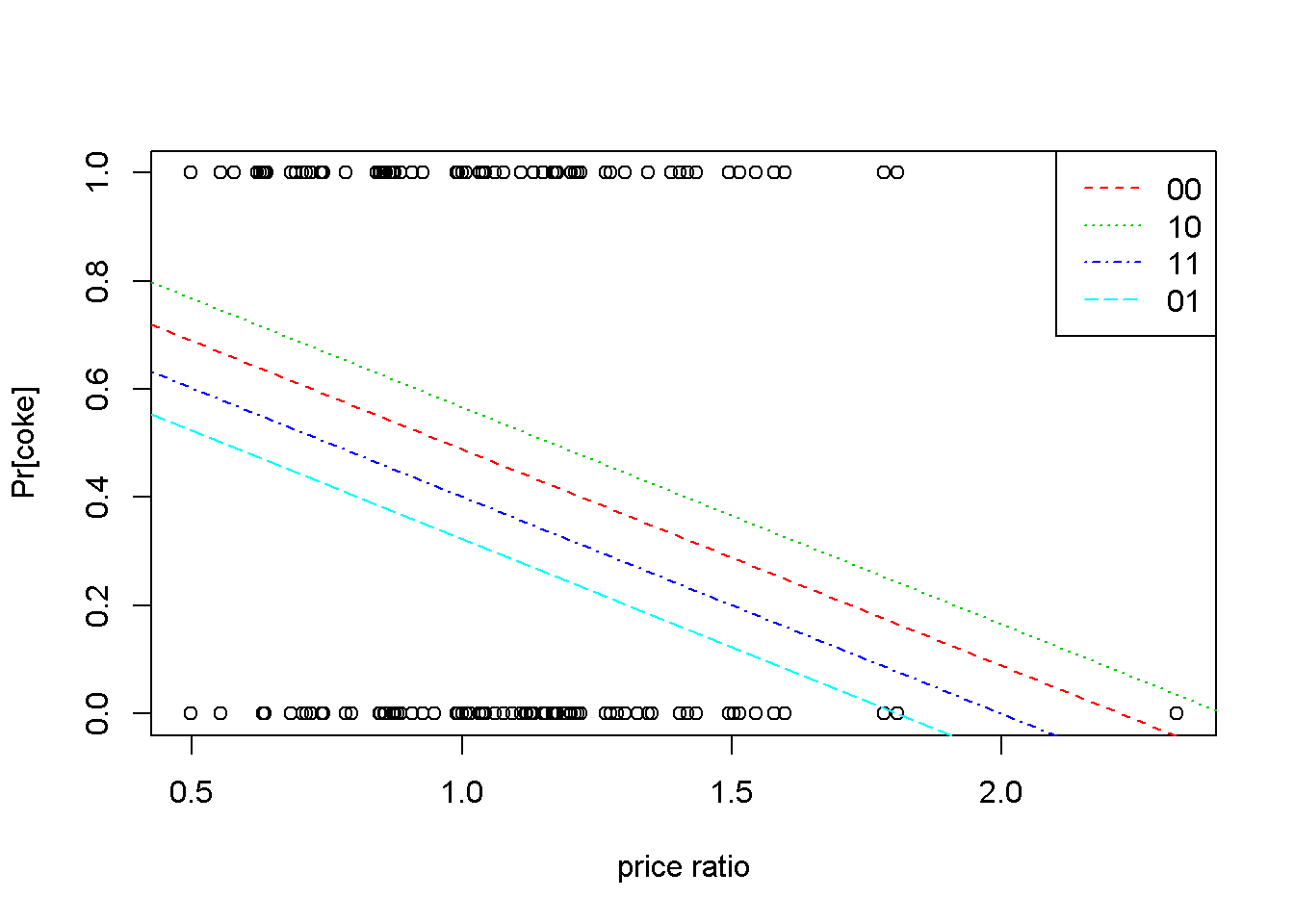

Figure 7.1: Linear probability: the ‘coke’ example

Figure 7.1 plots the probalility of choosing $coke$ with respect to the price ratio for the four possible combinations of the indicator variables $disp\_coke$ and $disp\_pepsi$ . In addition, the graph shows the observation points, all located at a height of either $0$ or $1$ . In the legend, the first digit is $0$ if $coke$ is not displayed and $1$ otherwise; the second digit does the same for $pepsi$ . Thus, the highest probability of choosing $coke$ for any given $pratio$ happens when $coke$ is displayed and $pepsi$ is not (the line marked $10$ ).

7.6 Treatment Effects

Treatment effects models aim at measuring the differences between a treatment group and a control group. The difference estimator is the simplest such a model and consists in constructing an indicator variable to distinguish between the two groups. Consider, for example, Equation $\ref{eq:diffes7}$ , where $d_{i}=1$ if observation $i$ belongs to the treatment group and $d_{i}=0$ otherwise.

$\begin{equation} y_{i}=\beta_{1}+\beta_{2}d_{i}+e_{i} \label{eq:diffes7} \end{equation}$

Thus, the expected value of the response is $\beta_{1}$ for the control group and $\beta_{1}+\beta_{2}$ for the treatment group. Put otherwise, the coefficient on the dummy variable represents the difference between the treatment and the control group. Moreover, it turns out that $b_{2}$ , the estimator of $\beta_{2}$ is equal to the difference between the sample averages of the two groups:

$\begin{equation} b_{2}=\bar y_{1}-\bar y_{0} \label{diffavg7} \end{equation}$

The dataset $star$ contains information on students from kindergarten to the third grade and was built to identify the determinants of student performance. Let us use this dataset for an example of a difference estimator, as well as an example of selecting just part of the variables and observations in a dataset.

The next piece of code presents a few new elements, that are used to select only a set of all the variables in the dataset, then to split the dataset in two parts: one for small classes, and one for regular classes. Lets look at these elements in the order in which they appear in the code. The function attach(datasetname) allows subsequent use of variable names without specifying from which database they come. While in general doing this is not advisable, I used it to simplify the next lines of code, which lists the variables I want to extract and assigns them to variable vars. As soon as I am done with splitting my dataset, I detach() the dataset to avoid subsequent confusion.

The line starregular is the one that actually retrieves the wanted variables and observations from the dataset. In essence, it picks from the dataset star the lines for which small==0 (see, no need for star$small as long as star is still attached). The same about the variable starsmall. Another novelty in the following code fragment is the use of the $R$ function stargazer() to vizualize a summary table instead of the usual function summary; stargazer shows a more familiar version of the summary statistics table.

# Project STAR, an application of the simple difference estimator
data("star", package="PoEdata")
attach(star)
vars <- c("totalscore","small","tchexper","boy",
          "freelunch","white_asian","tchwhite","tchmasters",
            "schurban","schrural")
starregular <- star[which(small==0),vars]
starsmall <- star[which(small==1),vars]
detach(star)
stargazer(starregular, type=.stargazertype, header=FALSE,
title="Dataset 'star' for regular classes")

**Dataset ‘star’ for regular classes**

Statistic	N	Mean	St. Dev.	Min	Max

totalscore	4,048	918.201	72.214	635	1,253
small	4,048	0.000	0.000	0	0
tchexper	4,028	9.441	5.779	0	27
boy	4,048	0.513	0.500	0	1
freelunch	4,048	0.486	0.500	0	1
white_asian	4,048	0.673	0.469	0	1
tchwhite	4,048	0.824	0.381	0	1
tchmasters	4,048	0.366	0.482	0	1
schurban	4,048	0.316	0.465	0	1
schrural	4,048	0.475	0.499	0	1

stargazer(starsmall, type=.stargazertype, header=FALSE,
title="Dataset 'star' for small classes")

**Dataset ‘star’ for small classes**

Statistic	N	Mean	St. Dev.	Min	Max

totalscore	1,738	931.942	76.359	747	1,253
small	1,738	1.000	0.000	1	1
tchexper	1,738	8.995	5.732	0	27
boy	1,738	0.515	0.500	0	1
freelunch	1,738	0.472	0.499	0	1
white_asian	1,738	0.685	0.465	0	1
tchwhite	1,738	0.862	0.344	0	1
tchmasters	1,738	0.318	0.466	0	1
schurban	1,738	0.306	0.461	0	1
schrural	1,738	0.463	0.499	0	1

The two tables titled “Dataset’star’…” display summary statistics for a number of variables in dataset ‘star’. The difference in the means of totalscore is equal to , which should be equal to the coefficient of the dummy variable small in Equation $\ref{eq:difesteq7}$ . (Note: the results for this dataset seem to be slightly different from $PoE4$ because the datasets used are of different sizes.)

$\begin{equation} totalscore=\beta_{1}+\beta_{2}small+e \label{eq:difesteq7} \end{equation}$

mod3 <- lm(totalscore~small, data=star)
b2 <- coef(mod3)[["small"]]

The difference estimated based on Equation $\ref{eq:difesteq7}$ is $b_{2}=13.740553$ , which coincides with the difference in means we calculated above.

If the students were randomly assigned to small or regular classes and the number of observations is large there is no need for additional regressors (there is no omitted variable bias if other regressors are not correlated with the variable small). In some instances, however, including other regressors may improve the difference estimator. Here is a model that includes a ‘teacher experience’ variable and some school characteristics (the students were randomized within schools, but schools were not randomized).

school <- as.factor(star$schid)#creates dummies for schools
mod4 <- lm(totalscore~small+tchexper, data=star)
mod5 <- lm(totalscore~small+tchexper+school, data=star)
b2n <- coef(mod4)[["small"]]
b2s <- coef(mod5)[["small"]]
anova(mod4, mod5)

Res.Df	RSS	Df	Sum of Sq	F	Pr(>F)
5763	30777461	NA	NA	NA	NA
5685	24072033	78	6705428	20.3025	0

By the introduction of school fixed effects the difference estimate have increased from $14.306725$ to $15.320602$ . The anova() function, which tests the equivalence of the two regressions yields a very low $p$ -value indicating that the difference between the two models is significant.

I have mentioned already, in the context of collinearity that a way to check if there is a relationship between an independent variable and the others is to regress that variable on the others and check the overall significance of the regression. The same method allows checking if the assignments to the treated and control groups are random. If we regress small on the other regressors and the assignment was random we should find no significant relationship.

mod6 <- lm(small~boy+white_asian+tchexper+freelunch, data=star)
kable(tidy(mod6), 
  caption="Checking random assignment in the 'star' dataset")

Table 7.7: Checking random assignment in the ‘star’ dataset
term	estimate	std.error	statistic	p.value
(Intercept)	0.325167	0.018835	17.264354	0.000000
boy	-0.000254	0.012098	-0.021014	0.983235
white_asian	0.012360	0.014489	0.853110	0.393634
tchexper	-0.002979	0.001055	-2.825242	0.004741
freelunch	-0.008800	0.013526	-0.650570	0.515350

fstat <- glance(mod6)$statistic
pf <- glance(mod6)$p.value

The $F$ -statistic of the model in Table 7.7 is $F=2.322664$ and its corresponding $p$ -value $0.054362$ , which shows that the model is overall insignificant at the 5% level or lower. The coefficients of the independent variables are insignificant or extremely small (the coefficient on $tchexper$ is statistically significant, but its marginal effect is a change in the probability that $small=1$ of about 0.3 percent). Again, these results provide fair evidence that the students’ assignment to small or regular classes was random.

7.7 The Difference-in-Differences Estimator

In many economic problems, which do not benefit from the luxury of random samples, the selection into one of the two groups is by choice, thus introducing a selection bias. The difference estimator is biased to the extent to which selection bias is present, therefore it is inadequate when selection bias may be present. The more complex difference-in-differences estimator is more appropriate in such cases. While the simple difference estimator assumes that before the treatment all units are identical or, at least, that the assignment to the treatment and control group is random, the difference-in-differences estimator takes into account any initial heterogeneity between the two groups.

The two ‘differences’ in the diference-in-differences estimator are: (i) the difference in the means of the treatment and control groups in the response variable after the treatment, and (ii) the difference in the means of the treatment and control groups in the response variable before the treatment. The ‘difference’ is between after and before.

Let us denote four averages of the response, as follows:

$\bar{y}_{T,\,A}$ Treatment, After
$\bar{y}_{C,\,A}$ Control, After
$\bar{y}_{T,\,B}$ Treatment, Before
$\bar{y}_{C,\,B}$ Control, Before

The difference-in-differences estimator is defined as in Equation $\ref{eq:dinddef7}$ .

$\begin{equation} \hat{\delta}= (\bar{y}_{T,\,A}-\bar{y}_{C,\,A})-(\bar{y}_{T,\,B}-\bar{y}_{C,\,B}) \label{eq:dinddef7} \end{equation}$

Instead of manually calculating the four means and their difference-in-differences, it is possible to estimate the difference-in-differences estimator and its statistical properties by running a regression that includes indicator variables for treatment and after and their interaction term. The advantage of a regression over simply using Equation $\ref{eq:dinddef7}$ is that the regression allows taking into account other factors that might influence the treatment effect. The simplest difference-in-differences regression model is presented in Equation $\ref{eq:dindgeneq7}$ , where $y_{it}$ is the response for unit $i$ in period $t$ . In the typical difference-in-differences model there are only two periods, before and after.

$\begin{equation} y_{it}=\beta_{1}+\beta_{2}T+\beta_{3}A+\delta T \times A+e_{it} \label{eq:dindgeneq7} \end{equation}$

With a litle algebra it can be seen that the coefficinet on the interaction term in Equation $\ref{eq:dindgeneq7}$ is exactly the difference-in-differences estimator defined in Equation $\ref{eq:dinddef7}$ . The following example calculates this estimator for the dataset $njmin3$ , where the response is $fte$ , the full-time equivalent employment, $d$ is the after dummy, with $d=1$ for the after period and $d=0$ for the before period, and $nj$ is the dummy that marks the treatment group ( $nj_{i}=1$ if unit $i$ is in New Jersey where the minimum wage law has been changed, and $nj_{i}=0$ if unit $i$ in Pennsylvania, where the minimum wage law has not changed). In other words, units (fast-food restaurants) located in New Jersey form the treatment group, and units located in Pennsylvania form the control group.

data("njmin3", package="PoEdata")
mod1 <- lm(fte~nj*d, data=njmin3)
mod2 <- lm(fte~nj*d+
             kfc+roys+wendys+co_owned, data=njmin3)
mod3 <- lm(fte~nj*d+
             kfc+roys+wendys+co_owned+
             southj+centralj+pa1, data=njmin3)
stargazer(mod1,mod2,mod3, 
          type=.stargazertype,
          title="Difference in Differences example",
          header=FALSE, keep.stat="n",digits=2 
#         single.row=TRUE, intercept.bottom=FALSE
          )

**Difference in Differences example**

	Dependent variable:

	fte
	(1)	(2)	(3)

nj	-2.89^**	-2.38^**	-0.91
	(1.19)	(1.08)	(1.27)

d	-2.17	-2.22	-2.21
	(1.52)	(1.37)	(1.35)

kfc		-10.45^***	-10.06^***
		(0.85)	(0.84)

roys		-1.62^*	-1.69^**
		(0.86)	(0.86)

wendys		-1.06	-1.06
		(0.93)	(0.92)

co_owned		-1.17	-0.72
		(0.72)	(0.72)

southj			-3.70^***
			(0.78)

centralj			0.01
			(0.90)

pa1			0.92
			(1.38)

nj:d	2.75	2.85^*	2.81^*
	(1.69)	(1.52)	(1.50)

Constant	23.33^***	25.95^***	25.32^***
	(1.07)	(1.04)	(1.21)


Observations	794	794	794

Note:	p<0.1; p<0.05; p<0.01

# t-ratio for delta, the D-in-D estimator:
tdelta <- summary(mod1)$coefficients[4,3]

The coefficient on the term $nj:d$ in the Table titled “Difference-in-Differences example” is $\delta$ , our difference-in-differences estimator. If we want to test the null hypothesis $H_{0}: \delta \geq 0$ , the rejection region is at the left tail; since the calculated $t$ , which is equal to $1.630888$ is positive, we cannot reject the null hypothesis. In other words, there is no evidence that an increased minimum wage reduces employment at fast-food restaurants.

Figure 7.2 displays the change of from the period before () to the period after the change in minimum wage () for both the treatment and the control groups. The line labeled “counterfactual” shows how the treatment group would have changed in the absence of the treatment, assuming its change would mirror the change in the control group. The graph is plotted using Equation $\ref{eq:dindgeneq7}$ .

b1 <- coef(mod1)[[1]]
b2 <- coef(mod1)[["nj"]]
b3 <- coef(mod1)[["d"]]
delta <- coef(mod1)[["nj:d"]]
C <- b1+b2+b3+delta
E <- b1+b3
B <- b1+b2
A <- b1
D <- E+(B-A)
# This creates an empty plot:
plot(1, type="n", xlab="period", ylab="fte", xaxt="n",
     xlim=c(-0.01, 1.01), ylim=c(18, 24))
segments(x0=0, y0=A, x1=1, y1=E, lty=1, col=2)#control
segments(x0=0, y0=B, x1=1, y1=C, lty=3, col=3)#treated
segments(x0=0, y0=B, x1=1, y1=D,      #counterfactual
         lty=4, col=4)
legend("topright", legend=c("control", "treated", 
    "counterfactual"), lty=c(1,3,4), col=c(2,3,4))
axis(side=1, at=c(0,1), labels=NULL)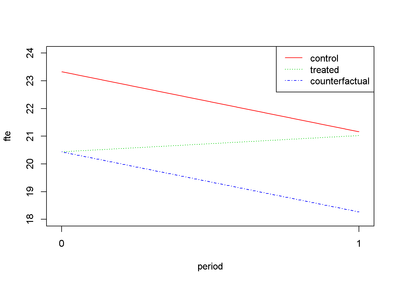

Figure 7.2: Difference-in-Differences for ‘njmin3’

7.8 Using Panel Data

The difference-in-differences method does not require that the same units be observed both periods, since it works with averages $\-$ before, and after. If we observe a number of units within the same time period, we construct a cross-section; if we construct different cross-sections in different periods we obtain a data structure named repeated cross-sections. Sometimes, however, we have information about the same units over several periods. A data structure in which the same (cross-sectional) units are observed over two or more periods is called a panel data and contains more information than a repeated cross-section. Let us re-consider the simplest equation (Equation $\ref{eq:dindnjmineq7}$ ), with the unit and time subscripts reflecting the panel data structure of the dataset. The time-invariant term $c_{i}$ has been added to reflect unobserved, individual-specific attributes.

$\begin{equation} fte_{it}=\beta_{1}+\beta_{2}nj_{i}+\beta_{3}d_{t}+\delta (nj_{i}\times d_{t})+c_{i} +e_{it} \label{eq:dindnjmineq7} \end{equation}$

In the dataset , some restaurants, belonging to either group have been observed both periods. If we restrict the dataset to only those restaurants we obtain a short (two period) panel data. Let us re-calculate the difference-in-differences estimator using this panel data. To do so, we notice that, if we write Equation $\ref{eq:dindnjmineq7}$ twice, once for each period and subtract the before from the after equation we obtain Equation $\ref{eq:paneldind7}$ , where the response, $dfte$ , is the after- minus- before difference in employment and the only regressor that remains is the treatment dummy, $nj$ , whose coefficient is $\delta$ , the very difference- in- differences estimator we are trying to estimate.

$\begin{equation} dfte_{i}=\alpha +\delta nj_{i}+u_{i} \label{eq:paneldind7} \end{equation}$

mod3 <- lm(demp~nj, data=njmin3)
kable(tidy(summary(mod3)), 
  caption="Difference in differences with panel data")

Table 7.8: Difference in differences with panel data
term	estimate	std.error	statistic	p.value
(Intercept)	-2.28333	0.731258	-3.12247	0.001861
nj	2.75000	0.815186	3.37346	0.000780

(smod3 <- summary(mod3))

## 
## Call:
## lm(formula = demp ~ nj, data = njmin3)
## 
## Residuals:
##    Min     1Q Median     3Q    Max 
## -39.22  -3.97   0.53   4.53  33.53 
## 
## Coefficients:
##             Estimate Std. Error t value Pr(>|t|)    
## (Intercept)   -2.283      0.731   -3.12  0.00186 ** 
## nj             2.750      0.815    3.37  0.00078 ***
## ---
## Signif. codes:  0 '***' 0.001 '**' 0.01 '*' 0.05 '.' 0.1 ' ' 1
## 
## Residual standard error: 8.96 on 766 degrees of freedom
##   (52 observations deleted due to missingness)
## Multiple R-squared:  0.0146, Adjusted R-squared:  0.0134 
## F-statistic: 11.4 on 1 and 766 DF,  p-value: 0.00078

$R^2=0.014639, \;\;\;F=11.380248, \;\;\;p=0.00078$

Table 7.8 shows a value of the estimated difference-in-differences coefficient very close to the one we estimated before. Its $t$ -statistic is still positive, indicating that the null hypothesis $H_{0}$ : “an increse in minimum wage increases employment” cannot be rejected.

7.9 R Practicum

7.9.1 Extracting Various Information

Here is a reminder on how to extract various results after fitting a linear model. The function names(lm.object) returns a list of the names of different items contained in the object. Suppose we run an lm() model and name it mod5. Then, mod5$name returns the item identified by the name. Like about everything in $R$ , there are many ways to extract values from an lm() object. I will present three objects that contain about everything we will need. These are the lm() object itself, summary(lm()), and the function glance(lm()) in package broom. The next code shows the name lists for all three objects and a few examples of extracting various statistics.

library(broom)
mod5 <- mod5 <- lm(wage~educ+black*female, data=cps4_small)
smod5 <- summary(mod5)
gmod5 <- glance(mod5) #from package 'broom'
names(mod5)

##  [1] "coefficients"  "residuals"     "effects"       "rank"         
##  [5] "fitted.values" "assign"        "qr"            "df.residual"  
##  [9] "xlevels"       "call"          "terms"         "model"

names(smod5)

##  [1] "call"          "terms"         "residuals"     "coefficients" 
##  [5] "aliased"       "sigma"         "df"            "r.squared"    
##  [9] "adj.r.squared" "fstatistic"    "cov.unscaled"

names(gmod5)

##  [1] "r.squared"     "adj.r.squared" "sigma"         "statistic"    
##  [5] "p.value"       "df"            "logLik"        "AIC"          
##  [9] "BIC"           "deviance"      "df.residual"

# Examples:
head(mod5$fitted.values)

##       1       2       3       4       5       6 
## 23.0605 19.5635 23.6760 18.5949 19.5635 19.5635

head(mod5$residuals)#head of residual vector

##         1         2         3         4         5         6 
## -4.360484 -8.063529 -8.636014  7.355080  4.466471  0.436471

smod5$r.squared

## [1] 0.208858

smod5$fstatistic # F-stat. and its degrees of freedom

##    value    numdf    dendf 
##  65.6688   4.0000 995.0000

gmod5$statistic #the F-statistic of the model

## [1] 65.6688

mod5$df.residual

## [1] 995

For some often used statistics, such as coefficients and their statistics, fitted values, or residuals there are specialized functions to extract them from regression results.

N <- nobs(mod5)
yhat <- fitted(mod5) # fitted values
ehat <- resid(mod5)  # estimated residuals
allcoeffs <- coef(mod5) # only coefficients, no statistics
coef(mod5)[[2]] #or:

## [1] 2.07039

coef(mod5)[["educ"]]

## [1] 2.07039

coeftest(mod5)# all coefficients and their statistics

## 
## t test of coefficients:
## 
##              Estimate Std. Error t value Pr(>|t|)    
## (Intercept)   -5.2812     1.9005  -2.779  0.00556 ** 
## educ           2.0704     0.1349  15.350  < 2e-16 ***
## black         -4.1691     1.7747  -2.349  0.01901 *  
## female        -4.7846     0.7734  -6.186 8.98e-10 ***
## black:female   3.8443     2.3277   1.652  0.09894 .  
## ---
## Signif. codes:  0 '***' 0.001 '**' 0.01 '*' 0.05 '.' 0.1 ' ' 1

# The 'tidy()' function is from the package 'broom':
tabl <- tidy(mod5) #this gives the same result as coeftest()
kable(tabl, caption=" Example of using the function 'tidy'")

Table 7.9: Example of using the function ‘tidy’
term	estimate	std.error	statistic	p.value
(Intercept)	-5.28116	1.900468	-2.77887	0.005557
educ	2.07039	0.134878	15.35009	0.000000
black	-4.16908	1.774714	-2.34916	0.019011
female	-4.78461	0.773414	-6.18635	0.000000
black:female	3.84429	2.327653	1.65158	0.098937

7.9.2 `ggplot2`, An Excellent Data Visualising Tool

The function ggplot in package ggplot2 is a very flexible plotting tool. For instance, it can assign different colours to different levels of an indicator variable. The following example uses the file utown to plot $price$ against $sqft$ using different colours for houses with swimming pool or for houses close to university.

library(ggplot2)
data("utown", package="PoEdata")
fpool <- as.factor(utown$pool)
futown <- as.factor(utown$utown)
ggplot(data = utown) + 
  geom_point(mapping = aes(x = sqft, y = price, 
  color = fpool, shape=fpool))
ggplot(data = utown) + 
  geom_point(mapping = aes(x = sqft, y = price, 
  color = futown, shape=futown))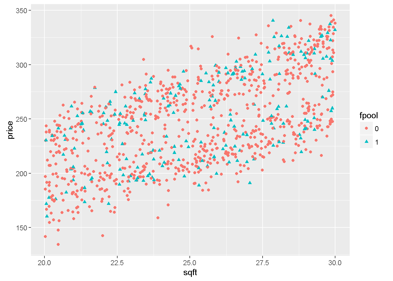

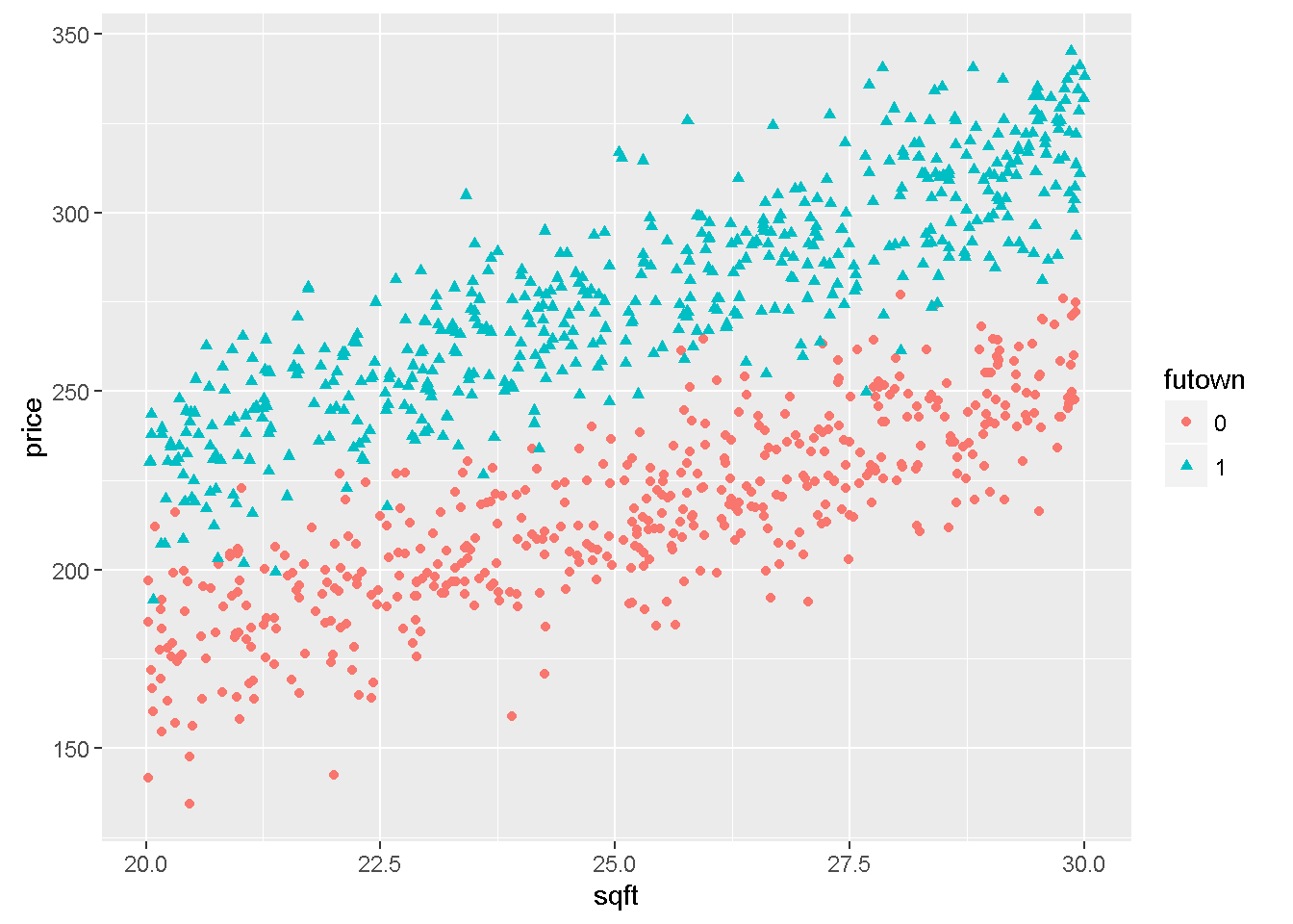
Figure 7.3: Graphs of dataset ‘utown’ using the ‘ggplot’ function

A brilliant, yet concise presentation of the ggplot() system can be found in (Grolemund and Wickham 2016), which I strongly recommend.

References

Hothorn, Torsten, Achim Zeileis, Richard W. Farebrother, and Clint Cummins. 2015. Lmtest: Testing Linear Regression Models. https://CRAN.R-project.org/package=lmtest.

Hlavac, Marek. 2015. Stargazer: Well-Formatted Regression and Summary Statistics Tables. https://CRAN.R-project.org/package=stargazer.

Grolemund, Garrett, and Hadley Wickham. 2016. R for Data Science. Online book. http://r4ds.had.co.nz/index.html.