Chapter 12 Time Series: Nonstationarity
rm(list=ls()) #Removes all items in Environment!
library(tseries) # for ADF unit root tests
library(dynlm)
library(nlWaldTest) # for the `nlWaldtest()` function
library(lmtest) #for `coeftest()` and `bptest()`.
library(broom) #for `glance(`) and `tidy()`
library(PoEdata) #for PoE4 datasets
library(car) #for `hccm()` robust standard errors
library(sandwich)
library(knitr) #for kable()
library(forecast)
New package: tseries (Trapletti and Hornik 2016).
A time series is nonstationary if its distribution, in particular its mean, variance, or timewise covariance change over time. Nonstationary time series cannot be used in regression models because they may create spurious regression, a false relationship due to, for instance, a common trend in otherwise unrelated variables. Two or more nonstationary series can still be part of a regression model if they are cointegrated, that is, they are in a stationary relationship of some sort.
We are concerned with testing time series for nonstationarity and finding out how can we transform nonstationary time series such that we can still use them in regression analysis.
data("usa", package="PoEdata")
usa.ts <- ts(usa, start=c(1984,1), end=c(2009,4),
               frequency=4)
Dgdp <- diff(usa.ts[,1])
Dinf <- diff(usa.ts[,"inf"])
Df <- diff(usa.ts[,"f"])
Db <- diff(usa.ts[,"b"])
usa.ts.df <- ts.union(gdp=usa.ts[,1], # package tseries
                      inf=usa.ts[,2],
                      f=usa.ts[,3],
                      b=usa.ts[,4],
                      Dgdp,Dinf,Df,Db,
                      dframe=TRUE)

plot(usa.ts.df$gdp)
plot(usa.ts.df$Dgdp)
plot(usa.ts.df$inf)
plot(usa.ts.df$Dinf)
plot(usa.ts.df$f)
plot(usa.ts.df$Df)
plot(usa.ts.df$b)
plot(usa.ts.df$Db)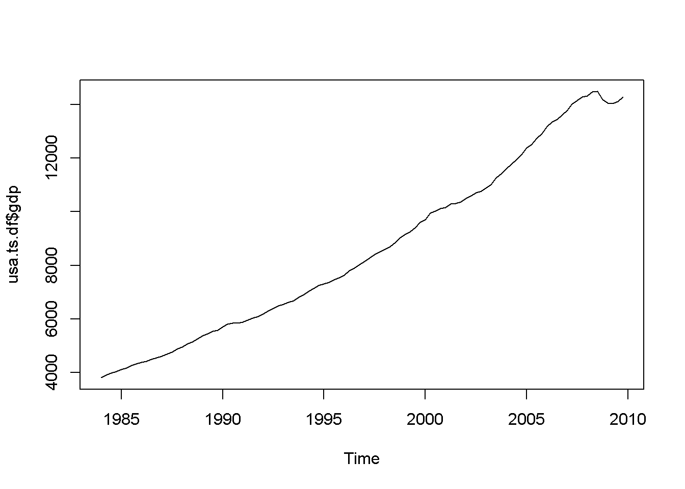
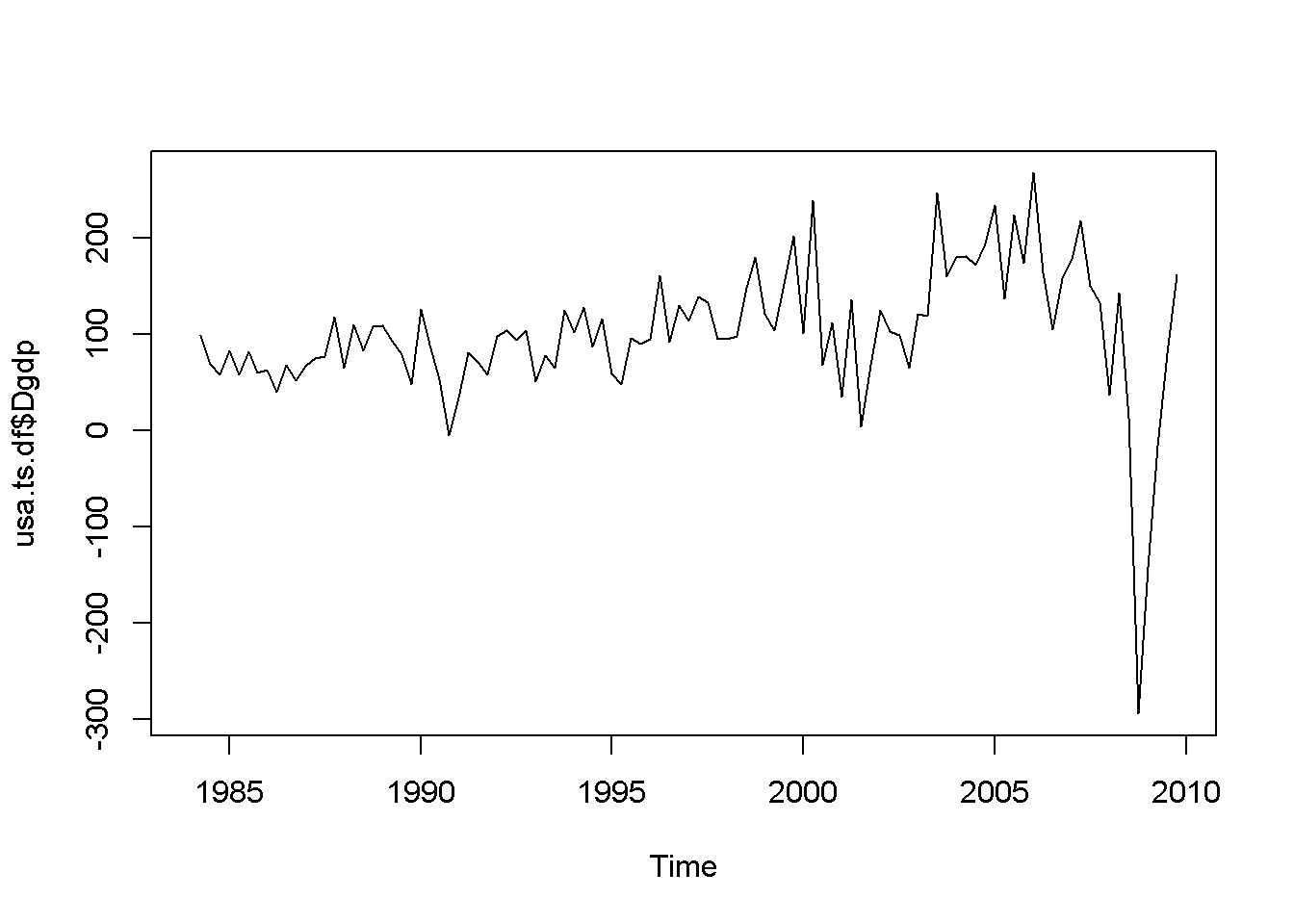
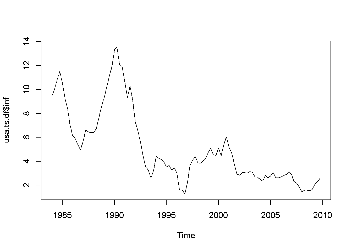
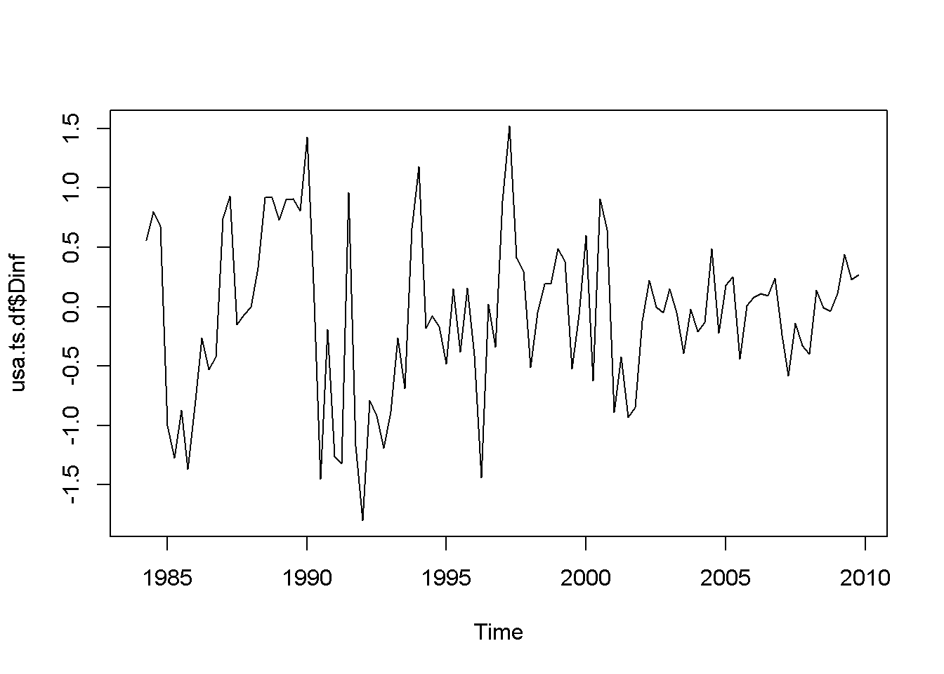

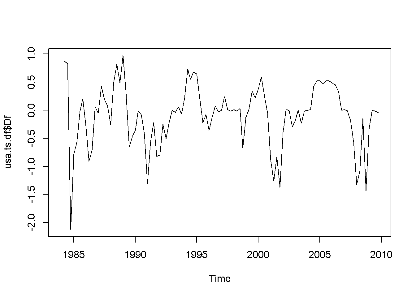

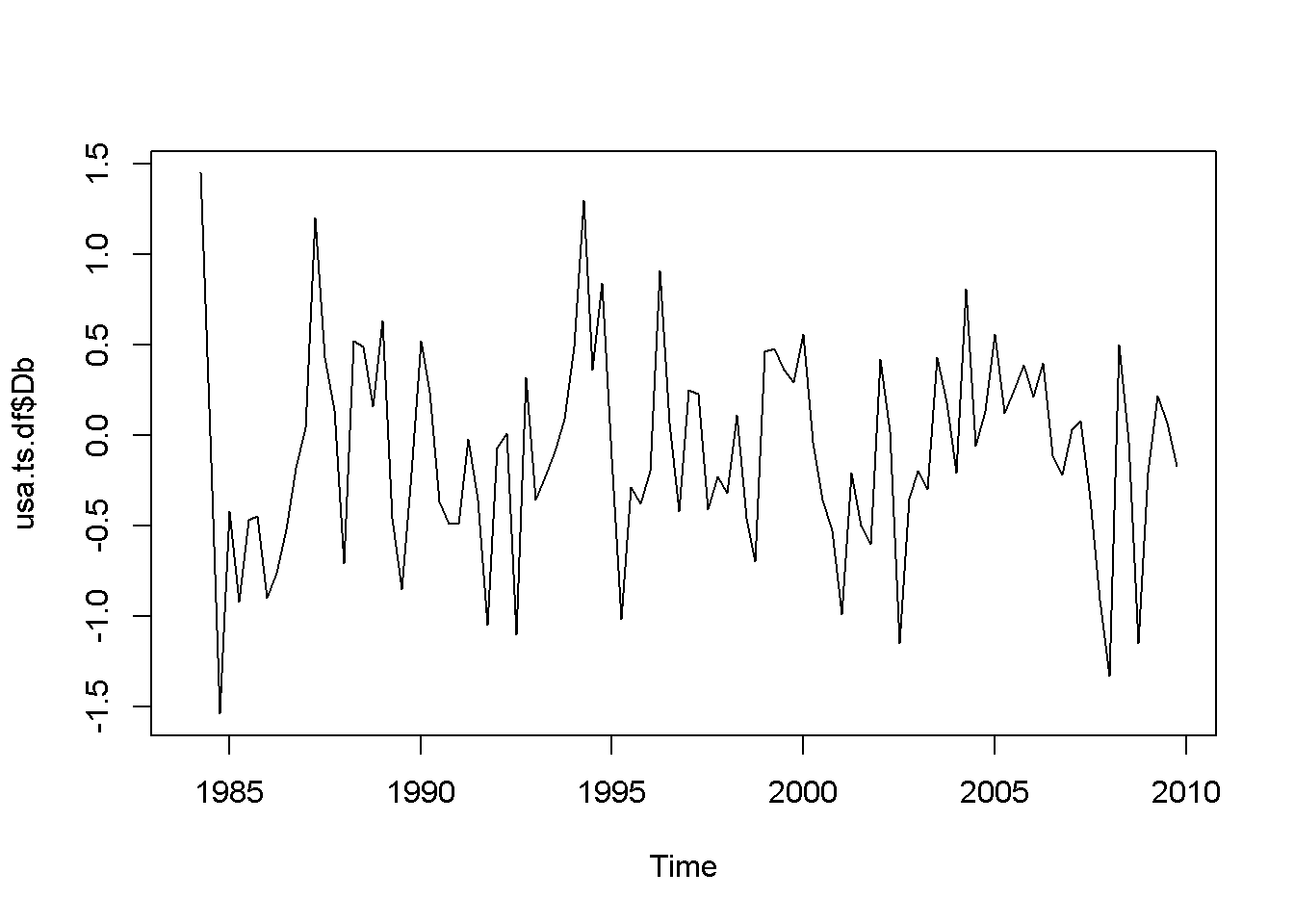
Figure 12.1: Various time series to illustrate nonstationarity
A novelty in the above code sequence is the use of the function ts.union, wich binds together several time series, with the possibility of constructing a data frame. Table 12.1 presents the head of this data frame.
kable(head(usa.ts.df),
caption="Time series data frame constructed with 'ts.union'")| gdp | inf | f | b | Dgdp | Dinf | Df | Db |
|---|---|---|---|---|---|---|---|
| 3807.4 | 9.47 | 9.69 | 11.19 | NA | NA | NA | NA |
| 3906.3 | 10.03 | 10.56 | 12.64 | 98.9 | 0.56 | 0.87 | 1.45 |
| 3976.0 | 10.83 | 11.39 | 12.64 | 69.7 | 0.80 | 0.83 | 0.00 |
| 4034.0 | 11.51 | 9.27 | 11.10 | 58.0 | 0.68 | -2.12 | -1.54 |
| 4117.2 | 10.51 | 8.48 | 10.68 | 83.2 | -1.00 | -0.79 | -0.42 |
| 4175.7 | 9.24 | 7.92 | 9.76 | 58.5 | -1.27 | -0.56 | -0.92 |
12.1 AR(1), the First-Order Autoregressive Model
An AR(1) stochastic process is defined by Equation \ref{eq:ar1def12}, where the error term is sometimes called “innovation” or “shock.”
\[\begin{equation} y_{t}=\rho y_{t-1}+\nu_{t},\;\;\;|\rho |<1 \label{eq:ar1def12} \end{equation}\]The AR(1) process is stationary if \(| \rho | <1\); when \(\rho=1\), the process is called random walk. The next code piece plots various AR(1) processes, with or without a constant, with or without trend (time as a term in the random process equation), with \(\rho\) lesss or equal to 1. The generic equation used to draw the diagrams is given in Equation \ref{eq:ar1generic12}.
\[\begin{equation} y_{t}=\alpha+\lambda t+\rho y_{t-1}+\nu_{t} \label{eq:ar1generic12} \end{equation}\]N <- 500
a <- 1
l <- 0.01
rho <- 0.7
set.seed(246810)
v <- ts(rnorm(N,0,1))
y <- ts(rep(0,N))
for (t in 2:N){
y[t]<- rho*y[t-1]+v[t]
}
plot(y,type='l', ylab="rho*y[t-1]+v[t]")
abline(h=0)
y <- ts(rep(0,N))
for (t in 2:N){
y[t]<- a+rho*y[t-1]+v[t]
}
plot(y,type='l', ylab="a+rho*y[t-1]+v[t]")
abline(h=0)
y <- ts(rep(0,N))
for (t in 2:N){
y[t]<- a+l*time(y)[t]+rho*y[t-1]+v[t]
}
plot(y,type='l', ylab="a+l*time(y)[t]+rho*y[t-1]+v[t]")
abline(h=0)
y <- ts(rep(0,N))
for (t in 2:N){
y[t]<- y[t-1]+v[t]
}
plot(y,type='l', ylab="y[t-1]+v[t]")
abline(h=0)
a <- 0.1
y <- ts(rep(0,N))
for (t in 2:N){
y[t]<- a+y[t-1]+v[t]
}
plot(y,type='l', ylab="a+y[t-1]+v[t]")
abline(h=0)
y <- ts(rep(0,N))
for (t in 2:N){
y[t]<- a+l*time(y)[t]+y[t-1]+v[t]
}
plot(y,type='l', ylab="a+l*time(y)[t]+y[t-1]+v[t]")
abline(h=0)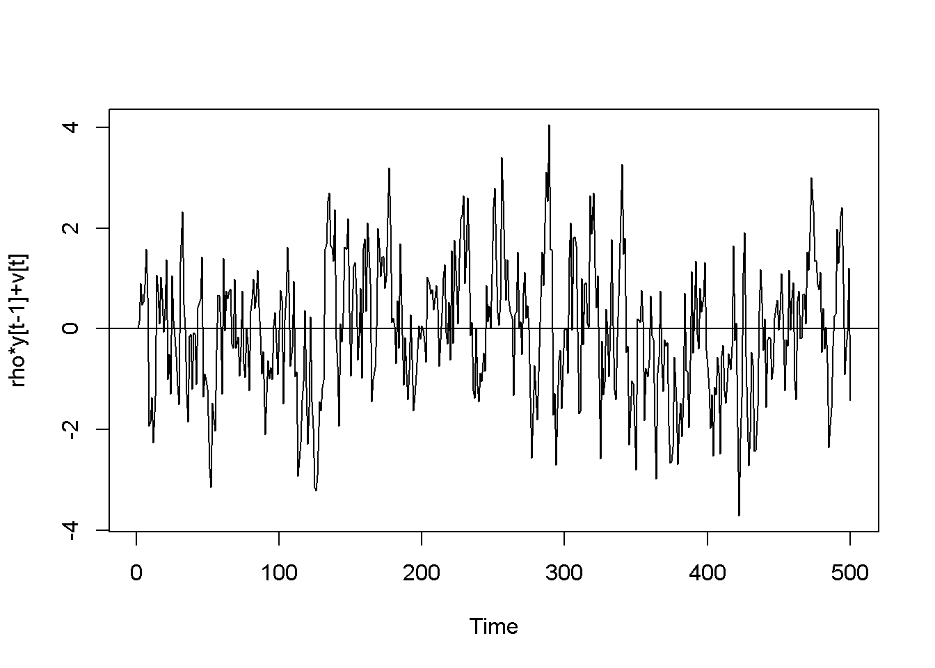
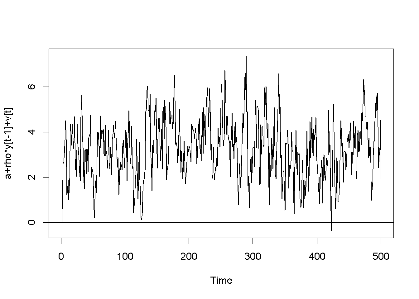
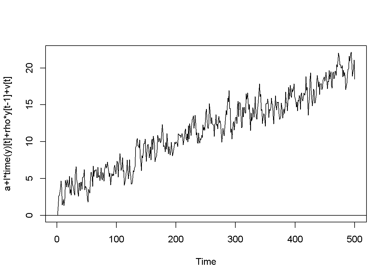
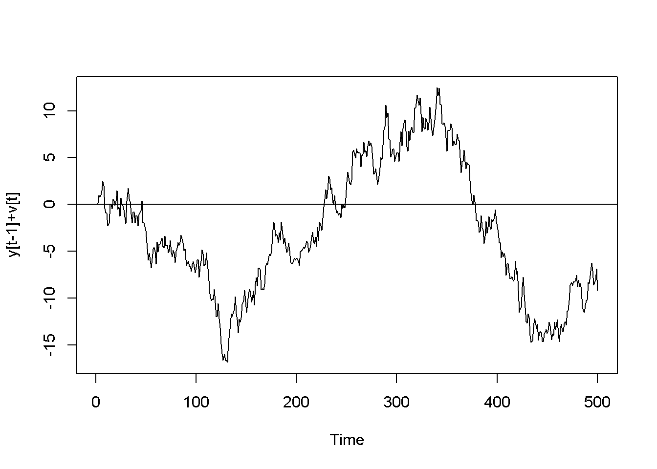
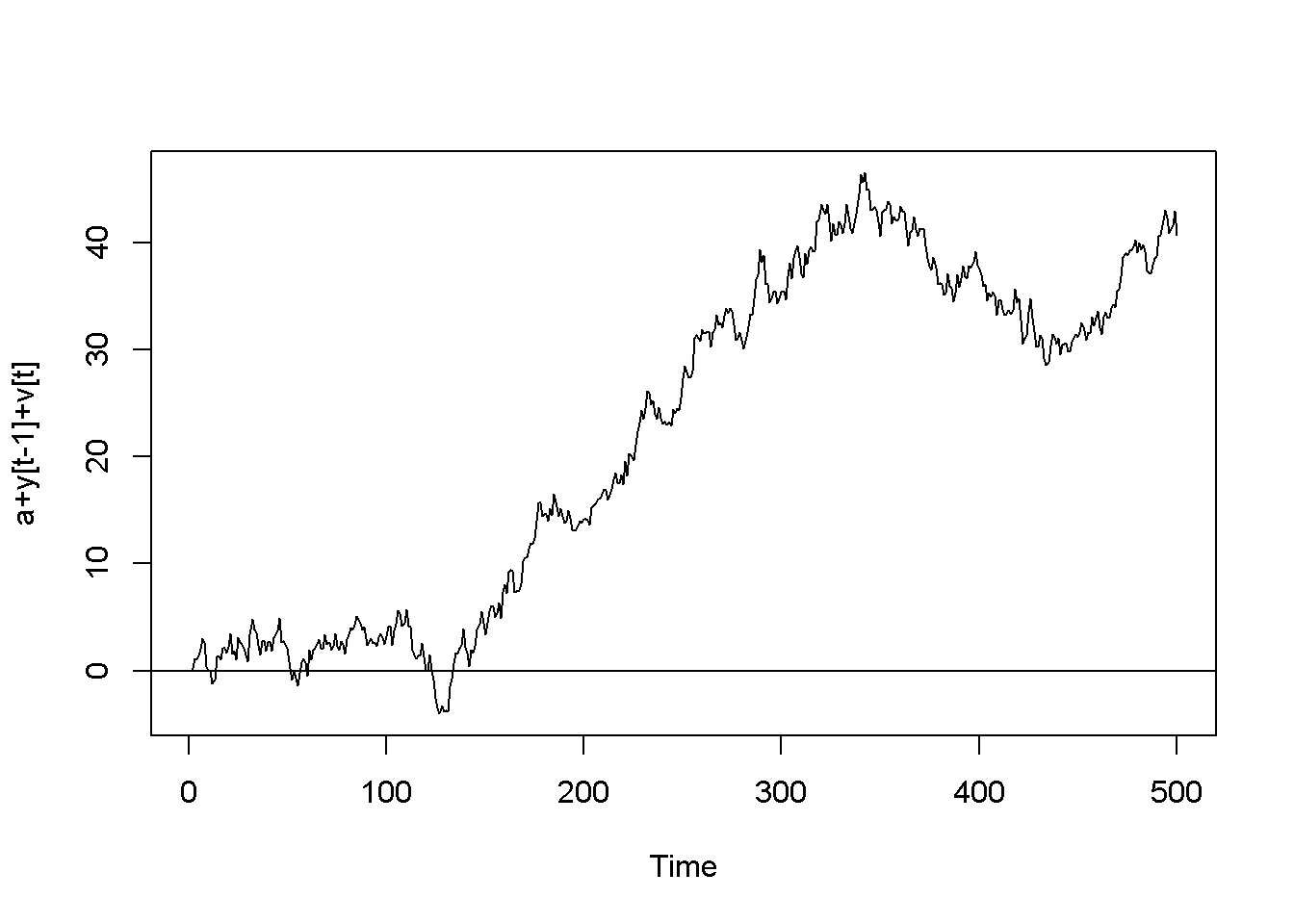
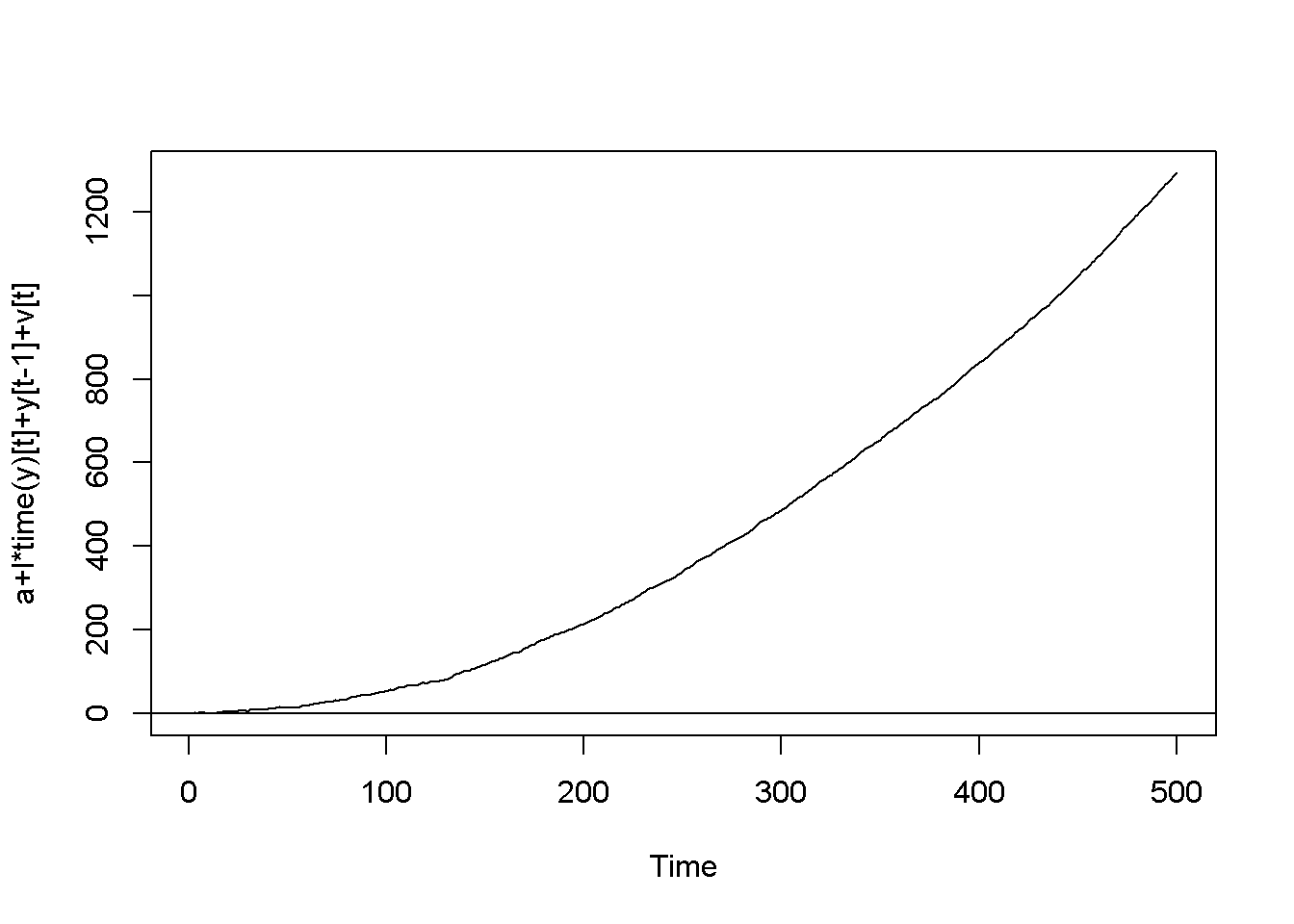
Figure 12.2: Artificially generated AR(1) processes with rho=0.7
12.2 Spurious Regression
Nonstationarity can lead to spurious regression, an apparent relationship between variables that are, in reality not related. The following code sequence generates two independent random walk processes, \(y\) and \(x\), and regresses \(y\) on \(x\).
T <- 1000
set.seed(1357)
y <- ts(rep(0,T))
vy <- ts(rnorm(T))
for (t in 2:T){
  y[t] <- y[t-1]+vy[t]
}

set.seed(4365)
x <- ts(rep(0,T))
vx <- ts(rnorm(T))
for (t in 2:T){
  x[t] <- x[t-1]+vx[t]
}
y <- ts(y[300:1000])
x <- ts(x[300:1000])
ts.plot(y,x, ylab="y and x")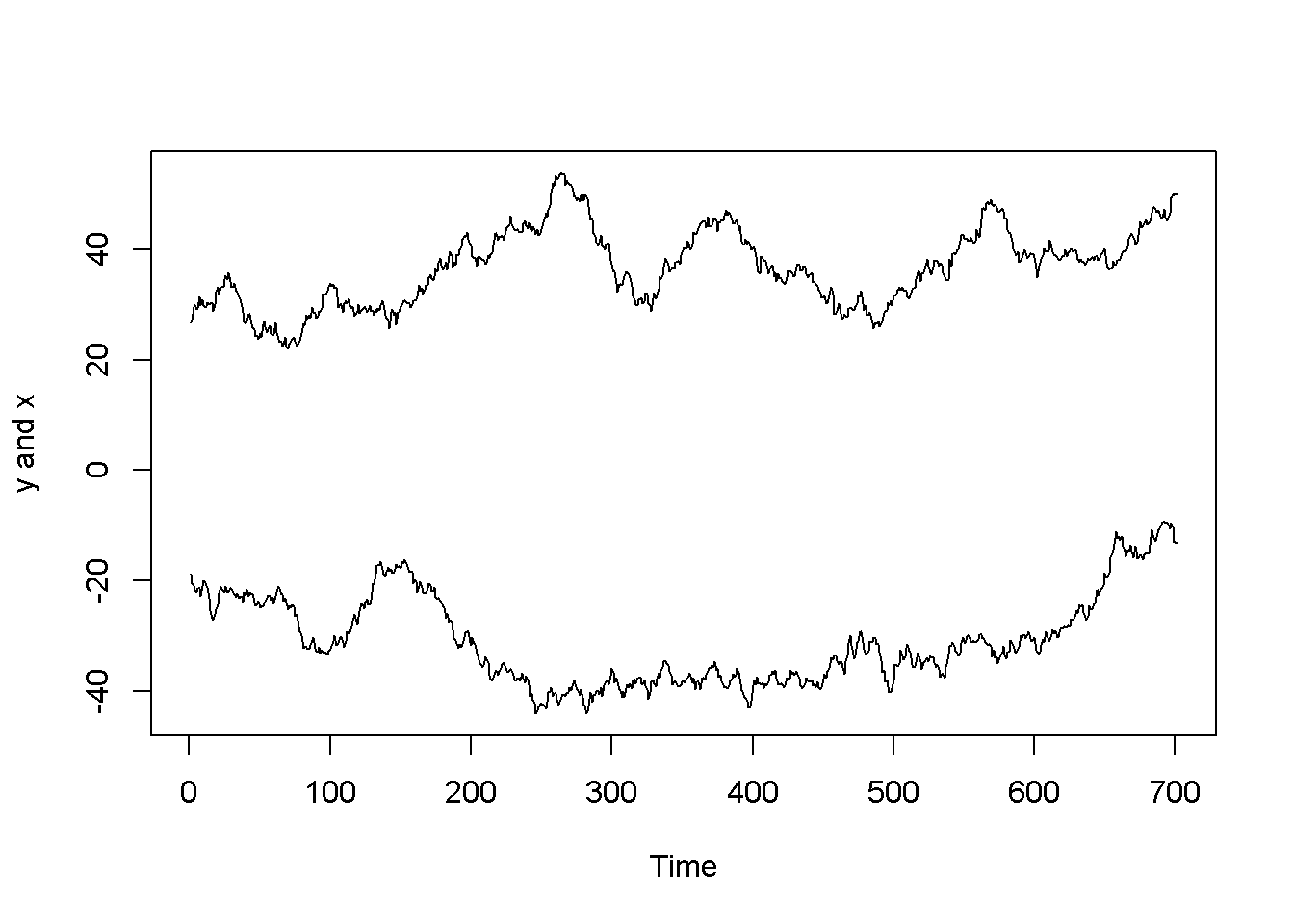
Figure 12.3: Artificially generated independent random variables
spurious.ols <- lm(y~x)
summary(spurious.ols)
##
## Call:
## lm(formula = y ~ x)
##
## Residuals:
## Min 1Q Median 3Q Max
## -12.55 -5.97 -2.45 4.51 24.68
##
## Coefficients:
## Estimate Std. Error t value Pr(>|t|)
## (Intercept) -20.3871 1.6196 -12.59 < 2e-16 ***
## x -0.2819 0.0433 -6.51 1.5e-10 ***
## ---
## Signif. codes: 0 '***' 0.001 '**' 0.01 '*' 0.05 '.' 0.1 ' ' 1
##
## Residual standard error: 7.95 on 699 degrees of freedom
## Multiple R-squared: 0.0571, Adjusted R-squared: 0.0558
## F-statistic: 42.4 on 1 and 699 DF, p-value: 1.45e-10The summary output of the regression shows a strong correlation between the two variables, thugh they have been generated independently. (Not any two randomly generated processes need to create spurious regression, though.) Figure 12.3 depicts the two time series, \(y\) and \(x\), and Figure 12.4 shows them in a scatterplot.
plot(x, y, type="p", col="grey")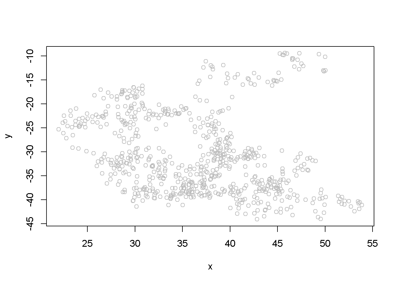
Figure 12.4: Scatter plot of artificial series y and x
12.3 Unit Root Tests for Stationarity
The Dickey-Fuller test for stationarity is based on an AR(1) process as defined in Equation \ref{eq:ar1def12}; if our time series seems to display a constant and trend, the basic equation is the one in Equation \ref{eq:ar1generic12}. According to the Dickey-Fuller test, a time series is nonstationary when \(\rho=1\), which makes the AR(1) process a random walk. The null and alternative hypotheses of the test is given in Equation \ref{eq:hypdftest12}.
\[\begin{equation} H_{0}: \rho=1, \;\;\; H_{A}: \rho <1 \label{eq:hypdftest12} \end{equation}\]The basic AR(1) equations mentioned above are transformed, for the purpose of the DF test into Equation \ref{eq:dftesteqn12}, with the transformed hypothesis shown in Equation \ref{eq:dftesthypo12}. Rejecting the DF null hypothesis implies that our time series is stationary.
\[\begin{equation} \Delta y_{t}=\alpha+\gamma y_{t-1}+\lambda t +\nu_{t} \label{eq:dftesteqn12} \end{equation}\] \[\begin{equation} H_{0}: \gamma =0, \;\;\;H_{A}: \gamma <0 \label{eq:dftesthypo12} \end{equation}\]An augmented DF test includes several lags of the variable tested; the number of lags to include can be assessed by examining the correlogram of the variable. The DF test can be of three types: with no constant and no trend, with constsnt and no trend, and, finally, with constant and trend. It is important to specify which DF test we want because the critical values are different for the three different types of the test. One decides which test to perform by examining a time series plot of the variable and determine if an imaginary regression line would have an intercept and a slope.
Let us apply the DF test to the \(f\) series in the \(usa\) dataset.
plot(usa.ts.df$f)
Acf(usa.ts.df$f)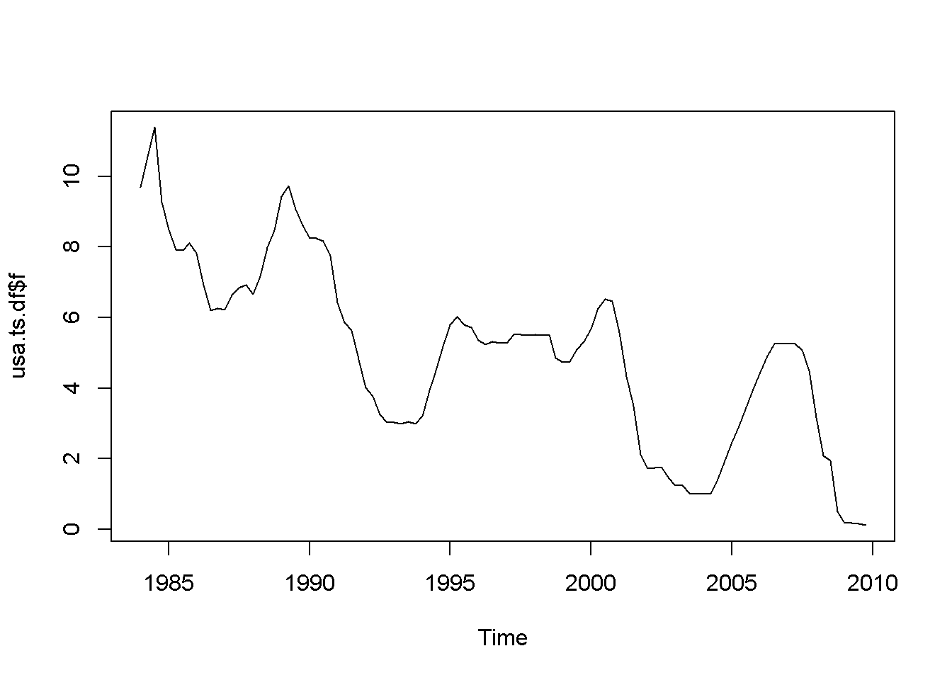
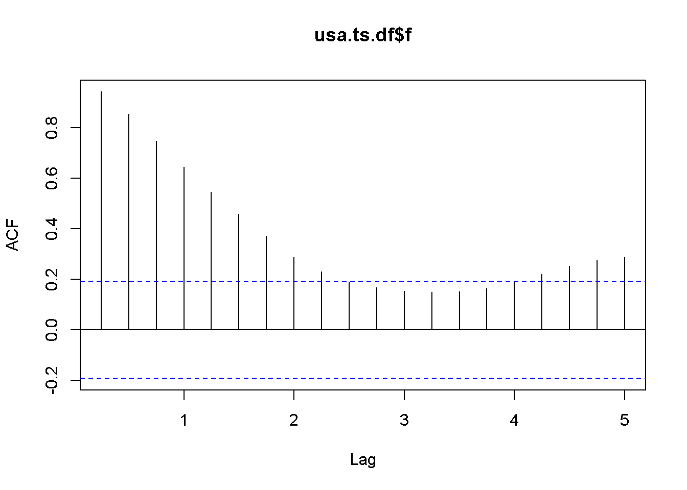
Figure 12.5: A plot and correlogram for series f in dataset usa
The time series plot in Figure 12.5 indicates both intercept and trend for our series, while the correlogram suggests including 10 lags in the DF test equation. Suppose we choose \(\alpha=0.05\) for the DF test. The adf.test function does not require specifying whether the test should be conducted with constant or trend, and if no value for the number of lags is given (the argument for the number of lags is k), \(R\) will calculate a value for it. I would recommend always taking a look at the series’ plot and correlogram.
adf.test(usa.ts.df$f, k=10)##
## Augmented Dickey-Fuller Test
##
## data: usa.ts.df$f
## Dickey-Fuller = -3.373, Lag order = 10, p-value = 0.0628
## alternative hypothesis: stationaryThe result of the test is a \(p\)-value greater than our chosen significance level of 0.05; therefore, we cannot reject the null hypothesis of nonstationarity.
plot(usa.ts.df$b)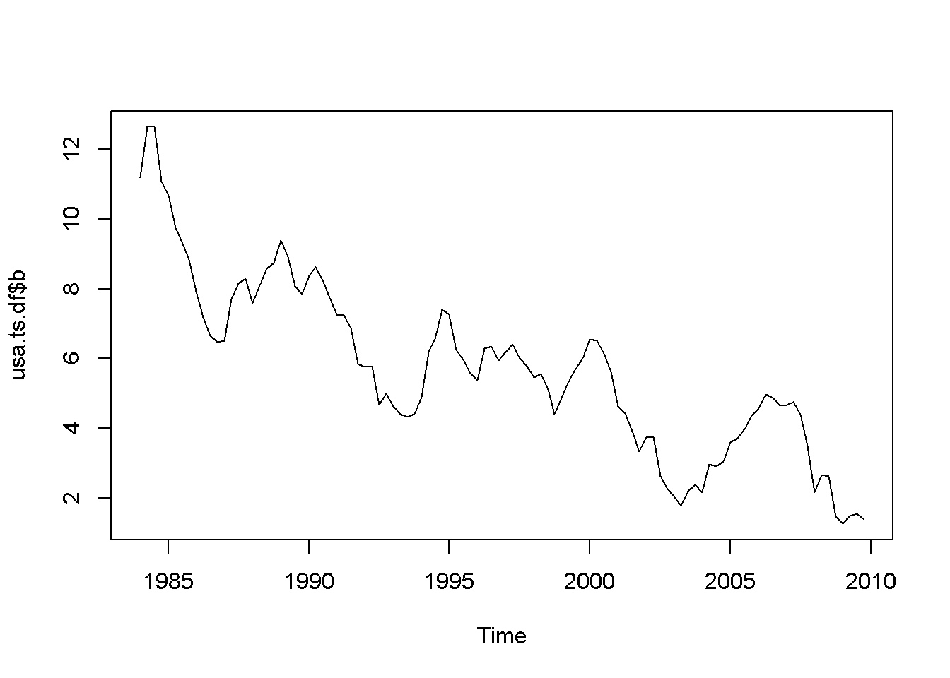
Acf(usa.ts.df$b)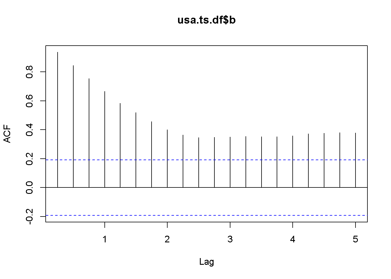
adf.test(usa.ts.df$b, k=10)##
## Augmented Dickey-Fuller Test
##
## data: usa.ts.df$b
## Dickey-Fuller = -2.984, Lag order = 10, p-value = 0.169
## alternative hypothesis: stationaryHere is a code to reproduce the results in the textbook.
f <- usa.ts.df$f
f.dyn <- dynlm(d(f)~L(f)+L(d(f)))
tidy(f.dyn)| term | estimate | std.error | statistic | p.value |
|---|---|---|---|---|
| (Intercept) | 0.172522 | 0.100233 | 1.72121 | 0.088337 |
| L(f) | -0.044621 | 0.017814 | -2.50482 | 0.013884 |
| L(d(f)) | 0.561058 | 0.080983 | 6.92812 | 0.000000 |
b <- usa.ts.df$b
b.dyn <- dynlm(d(b)~L(b)+L(d(b)))
tidy(b.dyn)| term | estimate | std.error | statistic | p.value |
|---|---|---|---|---|
| (Intercept) | 0.236873 | 0.129173 | 1.83376 | 0.069693 |
| L(b) | -0.056241 | 0.020808 | -2.70285 | 0.008091 |
| L(d(b)) | 0.290308 | 0.089607 | 3.23979 | 0.001629 |
A concept that is closely related to stationarity is order of integration, which is how many times we need to difference a series untill it becomes stationary. A series is I(0), that is, integrated of order \(0\) if it is already stationary (it is stationary in levels, not in differences); a series is I(1) if it is nonstationary in levels, but stationary in its first differences.
df <- diff(usa.ts.df$f)
plot(df)
Acf(df)
adf.test(df, k=2)
##
## Augmented Dickey-Fuller Test
##
## data: df
## Dickey-Fuller = -4.178, Lag order = 2, p-value = 0.01
## alternative hypothesis: stationary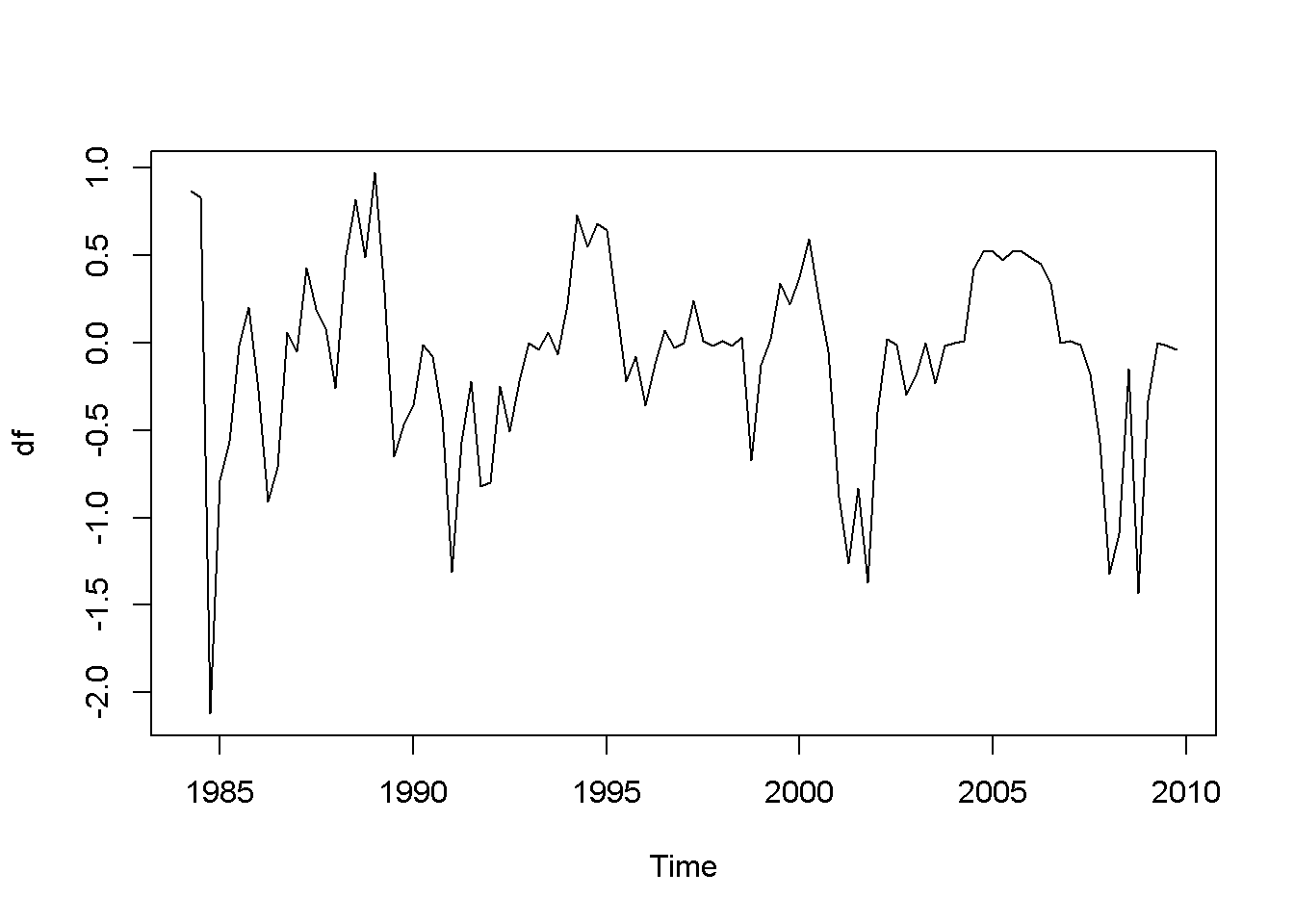
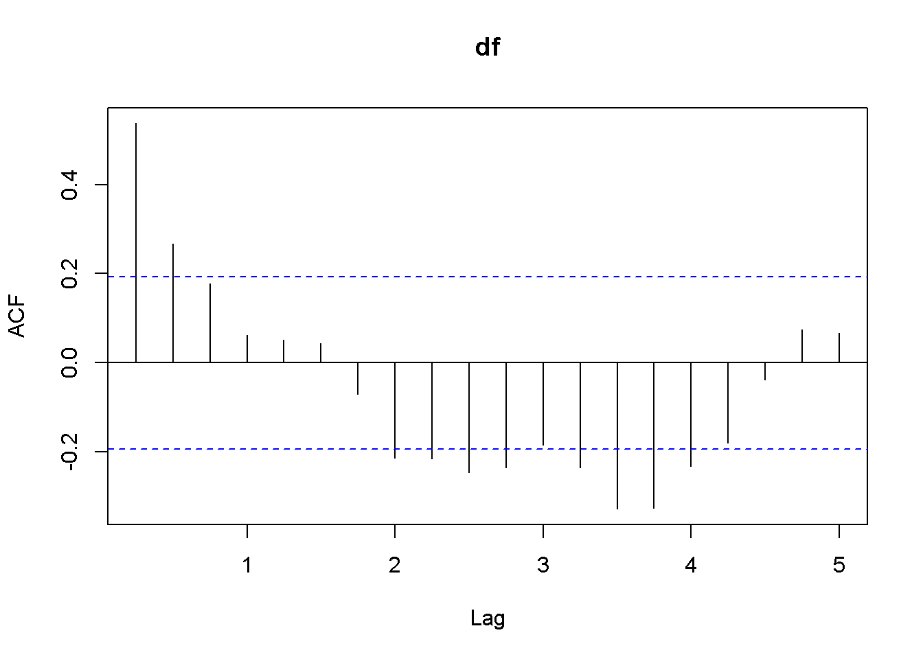
Figure 12.6: Plot and correlogram for series diff(f) in dataset usa
db <- diff(usa.ts.df$b)
plot(db)
Acf(db)
adf.test(db, k=1)
##
## Augmented Dickey-Fuller Test
##
## data: db
## Dickey-Fuller = -6.713, Lag order = 1, p-value = 0.01
## alternative hypothesis: stationary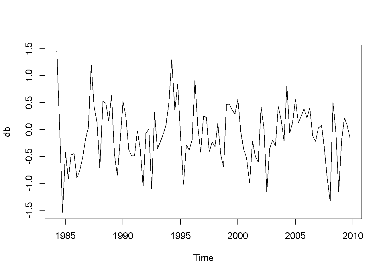
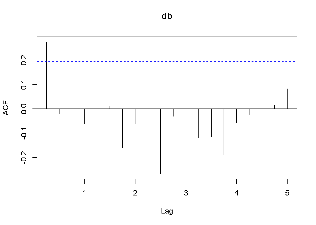
Figure 12.7: Plot and correlogram for series diff(b) in dataset usa
Both the plots and the DF tests indicate that the \(f\) and \(b\) series are stationary in first differences, which makes each of them integrated of order 1. The next code sequence reproduces the results in the textbook. Please note the term \((-1)\) in the dynlm command; it tells \(R\) that we do not want an intercept in our model. Figures 12.6 and 12.7 show plots of the differenced \(f\) and \(b\) series, respectively.
df.dyn <- dynlm(d(df)~L(df)-1)
db.dyn <- dynlm(d(db)~L(db)-1)
tidy(df.dyn)| term | estimate | std.error | statistic | p.value |
|---|---|---|---|---|
| L(df) | -0.446986 | 0.081462 | -5.48706 | 0 |
tidy(db.dyn)| term | estimate | std.error | statistic | p.value |
|---|---|---|---|---|
| L(db) | -0.701796 | 0.091594 | -7.66205 | 0 |
Function ndiffs() in the package forecast is a very convenient way of determining the order of integration of a series. The arguments of this function are x, a time series, alpha, the significacnce level of the test (0.05 by default), test= one of “kpss”, “adf”, or “pp”, which indicates the unit root test to be used; we have only studied the “adf” test.), and max.d= maximum number of differences. The output of this function is an integer, which is the order of integration of the time series.
ndiffs(f)## [1] 1ndiffs(b)## [1] 1As we have already found, the orders of integration for both \(f\) and \(b\) are 1.
12.4 Cointegration
Two series are cointegrated when their trends are not too far apart and are in some sense similar. This vague statement, though, can be made precise by conducting a cointegration test, which tests whether the residuals from regressing one series on the other one are stationary. If they are, the series are cointegrated. Thus, a cointegration test is in fact a Dickey-Fuler stationarity test on residuals, and its null hypothesis is of noncointegration. In other words, we would like to reject the null hypothesis in a cointegration test, as we wanted in a stationarity test.
Let us apply this method to determine the state of cointegration between the series \(f\) and \(b\) in dataset \(usa\).
fb.dyn <- dynlm(b~f)
ehat.fb <- resid(fb.dyn)
ndiffs(ehat.fb) #result: 1
## [1] 1output <- dynlm(d(ehat.fb)~L(ehat.fb)+L(d(ehat.fb))-1) #no constant
foo <- tidy(output)
foo| term | estimate | std.error | statistic | p.value |
|---|---|---|---|---|
| L(ehat.fb) | -0.224509 | 0.053504 | -4.19613 | 0.000059 |
| L(d(ehat.fb)) | 0.254045 | 0.093701 | 2.71124 | 0.007891 |
The relevant statistic is \(\tau = -4.196133\), which is less than \(-3.37\), the relevant critical value for the cointegration test. In conclusion, we reject the null hypothesis that the residuals have unit roots, therefore the series are cointegrated.
\(R\) has a special function to perform cointegration tests, function po.test in package tseries. (The name comes from the method it uses, which is called “Phillips-Ouliaris.”) The main argument of the function is a matrix having in its first column the dependent variable of the cointegration equation and the independent variables in the other columns. Let me illustrate its application in the case of the same series \(fb\) and \(f\).
bfx <- as.matrix(cbind(b,f), demean=FALSE)
po.test(bfx)
##
## Phillips-Ouliaris Cointegration Test
##
## data: bfx
## Phillips-Ouliaris demeaned = -20.51, Truncation lag parameter = 1,
## p-value = 0.0499The PO test marginally rejects the null of no cointegration at the 5 percent level.
12.5 The Error Correction Model
A relationship between cointegrated I(1) variables is a long run relationship, while a relationship between I(0) variables is a short run one. The short run error correction model combines, in some sense, short run and long run effects. Starting from an ARDL(1,1) model (Equation \ref{eq:ardl11error12}) and assuming that there is a steady state (long run) relationship between \(y\) and \(x\), one can derive the error correction model in Equation \ref{eq:errorcorreqn12}, where more lagged differences of \(x\) may be necessary to eliminate autocorrelation.
\[\begin{equation} y_{t}=\delta+\theta_{1}y_{t-1}+\delta_{0}x_{t}+\delta_{1}x_{t-1}+\nu_{t} \label{eq:ardl11error12} \end{equation}\] \[\begin{equation} \Delta y_{t}=-\alpha (y_{t-1}-\beta_{1}-\beta_{2}x_{t-1})+\delta_{0}\Delta x_{t}+\nu_{t} \label{eq:errorcorreqn12} \end{equation}\]In the case of the US bonds and funds example, the error correction model can be constructed as in Equation \ref{eq:bferrorcorrection12}.
\[\begin{equation} \Delta b_{t}=-\alpha (b_{t-1}-\beta_{1}-\beta_{2}f_{t-1})+\delta_{0}\Delta \, f_{t}+ \delta_{1}\Delta \, f_{t-1} + \nu_{t} \label{eq:bferrorcorrection12} \end{equation}\]The \(R\) function that estimates a nonlinear model such as the one in Equation \ref{eq:bferrorcorrection12} is nls, which requires three main argumants: a formula, which is the regression model to be estimated written using regular text mathematical operators, a start= list of guessed or otherwise approximated values of the estimated parameters to initiate a Gauss-Newton numerical optimization process, and data= a data frame, list, or environment data source. Please note that data cannot be a matrix.
In the next code sequence, the initial values of the parameters have been determined by estimating Equation \ref{eq:ardl11error12} with \(b\) and \(f\) replacing \(y\) and \(x\).
b.ols <- dynlm(L(b)~L(f))
b1ini <- coef(b.ols)[[1]]
b2ini <- coef(b.ols)[[2]]
d.ols <- dynlm(b~L(b)+f+L(f))
aini <- 1-coef(d.ols)[[2]]
d0ini <- coef(d.ols)[[3]]
d1ini <- coef(d.ols)[[4]]
Db <- diff(b)
Df <- diff(f)
Lb <- lag(b,-1)
Lf <- lag(f,-1)
LDf <- lag(diff(f),-1)
bfset <- data.frame(ts.union(cbind(b,f,Lb,Lf,Db,Df,LDf)))
formula <- Db ~ -a*(Lb-b1-b2*Lf)+d0*Df+d1*LDf
bf.nls <- nls(formula, na.action=na.omit, data=bfset,
          start=list(a=aini, b1=b1ini, b2=b2ini,
                     d0=d0ini, d1=d1ini))
kable(tidy(bf.nls),
caption="Parameter estimates in the error correction model")| term | estimate | std.error | statistic | p.value |
|---|---|---|---|---|
| a | 0.141877 | 0.049656 | 2.85720 | 0.005230 |
| b1 | 1.429188 | 0.624625 | 2.28807 | 0.024304 |
| b2 | 0.776557 | 0.122475 | 6.34052 | 0.000000 |
| d0 | 0.842463 | 0.089748 | 9.38697 | 0.000000 |
| d1 | -0.326845 | 0.084793 | -3.85463 | 0.000208 |
The error correction model can also be used to test the two series for cointegration. All we need to do is to test the errors of the correction part embedded in Equation \ref{eq:bferrorcorrection12} for stationarity. The estimated errors are given by Equation \ref{eq:embederrors12}.
\[\begin{equation} \hat{e}_{t-1}=b_{t-1}-\beta_{1}-\beta_{2}f_{t-1} \label{eq:embederrors12} \end{equation}\]ehat <- bfset$Lb-coef(bf.nls)[[2]]-coef(bf.nls)[[3]]*bfset$Lf
ehat <- ts(ehat)
ehat.adf <- dynlm(d(ehat)~L(ehat)+L(d(ehat))-1)
kable(tidy(ehat.adf),
caption="Stationarity test within the error correction model")| term | estimate | std.error | statistic | p.value |
|---|---|---|---|---|
| L(ehat) | -0.168488 | 0.042909 | -3.92668 | 0.000158 |
| L(d(ehat)) | 0.179486 | 0.092447 | 1.94149 | 0.055013 |
foo <- tidy(ehat.adf)To test for cointegration, one should compare the \(t\)-ratio of the lagged term shown as ‘statistic’ in Equation 12.3, \(t=-3.927\) to the critical value of \(-3.37\). The result is to reject the null of no cointegration, which means the series are cointegrated.
References
Trapletti, Adrian, and Kurt Hornik. 2016. Tseries: Time Series Analysis and Computational Finance. https://CRAN.R-project.org/package=tseries.