Chapter 16 Qualitative and LDV Models
rm(list=ls()) #Removes all items in Environment!
library(nlWaldTest) # for the `nlWaldtest()` function
library(lmtest) #for `coeftest()` and `bptest()`.
library(broom) #for `glance(`) and `tidy()`
library(PoEdata) #for PoE4 datasets
library(car) #for `hccm()` robust standard errors
library(sandwich)
library(knitr) #for `kable()`
library(forecast)
library(AER)
library(xtable)
16.1 The Linear Probability Model
Suppose the response variable is binary, as defined in Equation \ref{eq:binaryydef16}.
\[\begin{equation} y=1\;\; \text {if an individual chooses to buy a house}\\ y=0\;\; \text {if an individual chooses not to buy} \label{eq:binaryydef16} \end{equation}\]The linear probability model has the general form is shown in Equation \ref{eq:lpmgen16}. \(E(y)\) is the probability that the response variable takes the value of \(1\); therefore, a predicted value of \(y\) is a prediction for the probability that \(y=1\).
\[\begin{equation} y=E(y)+e=\beta_{1}+\beta_{2}x_{2}+...+\beta_{k}x_{k}+e \label{eq:lpmgen16} \end{equation}\]16.2 The Probit Model
The probit model assumes a nonlinear relationship between the response variable and regressors, this relationship being the cumulative distribution function of the normal distribution (see Equation \ref{eq:probitdef16} and Figure 16.1, left).
\[\begin{equation} p=P[y=1]=E(y|x)=\Phi (\beta_{1}+\beta_{2}x) \label{eq:probitdef16} \end{equation}\]The slope of the regression curve is not constant, but is given by the standard normal density function (Figure 16.1, right); the slope can be calculated using Equation \ref{eq:probitslope16}.
\[\begin{equation} \frac{dp}{dx}=\phi(\beta_{1}+\beta_{2}x)\beta_{2} \label{eq:probitslope16} \end{equation}\]Predictions of the probability that \(y=1\) are given by Equation \ref{eq:probitpredict16}.
\[\begin{equation} \hat p =\Phi(\hat \beta_{1}+\hat \beta_{2}x) \label{eq:probitpredict16} \end{equation}\]x <- seq(-3,3, .2)
plot(x, pnorm(x), type="l", xlab="b1+b2x", ylab="P[y=1]")
plot(x, dnorm(x), type="l")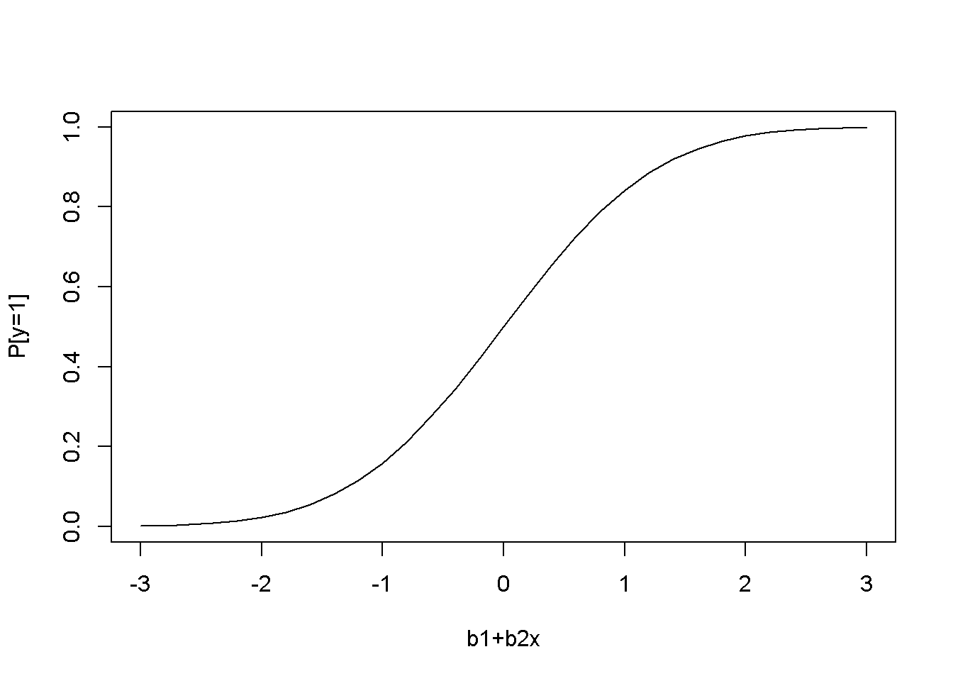
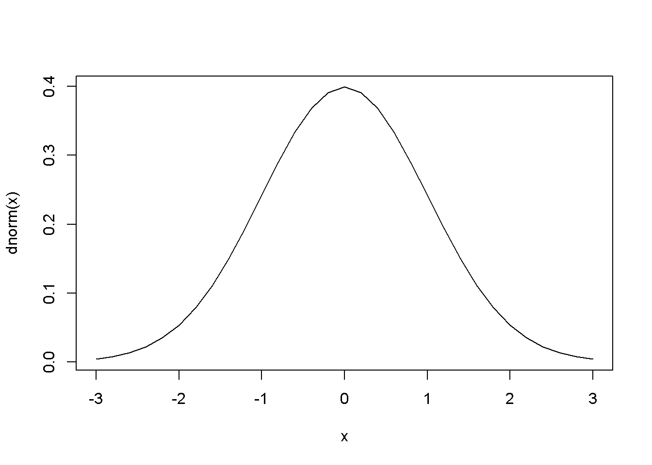
Figure 16.1: The shape of the probit function is the standard normal distribution
16.3 The Transportation Example
The dataset \(transport\) containes \(N=21\) observations of transportation chioces (\(auto=1\) if individual \(i\) chooses \(auto\) and \(0\) if individual \(i\) chooses \(bus\)). The choice depends on the difference in time between the two means of transportation, \(dtime=(bustime-autotime)\div 10\).
The \(R\) function to estimate a probit model is glm, with the family argument equal to binomial(link="probit"). The glm function has the following general structure:
glm(formula, family, data, …)
data("transport", package="PoEdata")
auto.probit <- glm(auto~dtime, family=binomial(link="probit"),
                   data=transport)
kable(tidy(auto.probit), digits=4, align='c', caption=
"Transport example, estimated by probit")| term | estimate | std.error | statistic | p.value |
|---|---|---|---|---|
| (Intercept) | -0.0644 | 0.4007 | -0.1608 | 0.8722 |
| dtime | 0.3000 | 0.1029 | 2.9154 | 0.0036 |
Equation \ref{eq:probitslope16} can be used to calculate partial effects of an increase in \(dtime\) by one unit (10 minutes). The following code lines calculate this effect at \(dtime=2\) (time difference of 20 minutes).
xdtime <- data.frame(dtime=2)
predLinear <- predict(auto.probit, xdtime,
                data=transport, type="link")
DpDdtime <- coef(auto.probit)[[2]]*dnorm(predLinear)
DpDdtime
## 1
## 0.10369Predictions can be calculated using the function predict, which has the following general form:
predict(object, newdata = NULL, type = c(“link”, “response”, “terms”), se.fit = FALSE, dispersion = NULL, terms = NULL, na.action = na.pass, …)
The optional argument newdata must be a data frame containing the new values of the regressors for which the prediction is desired; if missing, prediction is calculated for all observations in the sample.
Here is how to calculate the predicted probability of choosing \(auto\) when the time difference is 30 minutes (\(dtime=3\)):
xdtime <- data.frame(dtime=3)
predProbit <- predict(auto.probit, xdtime,
              data=transport, type="response")
predProbit
## 1
## 0.798292The marginal effect at the average predicted value can be determined as follows:
avgPredLinear <- predict(auto.probit, type="link")
avgPred <- mean(dnorm(avgPredLinear))
AME <- avgPred*coef(auto.probit)
AME
## (Intercept) dtime
## -0.0103973 0.048406916.4 The Logit Model for Binary Choice
This is very similar to the probit model, with the difference that logit uses the logistic function \(\Lambda\) to link the linear expression \(\beta_{1}+\beta_{2}x\) to the probability that the response variable is equal to \(1\). Equations \ref{eq:logitdefA16} and \ref{eq:logitdefB16} give the defining expressions of the logit model (the two expressions are equivalent).
\[\begin{equation} p=\Lambda (\beta_{1}+\beta_{2}x)=\frac{1}{1+e^{-( \beta_{1}+\beta_{2}x)}} \label{eq:logitdefA16} \end{equation}\] \[\begin{equation} p=\frac{exp(\beta_{1}+\beta_{2}x)}{1+exp(\beta_{1}+\beta_{2}x)} \label{eq:logitdefB16} \end{equation}\]Equation \ref{eq:MargEffLogit} gives the marginal effect of a change in the regressor \(x_{k}\) on the probability that \(y=1\).
\[\begin{equation} \frac{\partial p}{\partial x_{k}}=\beta_{k}\Lambda (1-\Lambda) \label{eq:MargEffLogit} \end{equation}\]data("coke", package="PoEdata")
coke.logit <- glm(coke~pratio+disp_coke+disp_pepsi,
data=coke, family=binomial(link="logit"))
kable(tidy(coke.logit), digits=5, align="c",
caption="Logit estimates for the 'coke' dataset")| term | estimate | std.error | statistic | p.value |
|---|---|---|---|---|
| (Intercept) | 1.92297 | 0.32582 | 5.90200 | 0.00000 |
| pratio | -1.99574 | 0.31457 | -6.34437 | 0.00000 |
| disp_coke | 0.35160 | 0.15853 | 2.21781 | 0.02657 |
| disp_pepsi | -0.73099 | 0.16783 | -4.35551 | 0.00001 |
coke.LPM <- lm(coke~pratio+disp_coke+disp_pepsi,
              data=coke)
coke.probit <- glm(coke~pratio+disp_coke+disp_pepsi,
              data=coke, family=binomial(link="probit"))
stargazer(coke.LPM, coke.probit, coke.logit,
  header=FALSE,
  title="Three binary choice models for the 'coke' dataset",
  type=.stargazertype,
  keep.stat="n",digits=4, single.row=FALSE,
  intercept.bottom=FALSE,
  model.names=FALSE,
column.labels=c("LPM","probit","logit"))| Dependent variable: | |||
| coke | |||
| LPM | probit | logit | |
| (1) | (2) | (3) | |
| Constant | 0.8902*** | 1.1080*** | 1.9230*** |
| (0.0655) | (0.1925) | (0.3258) | |
| pratio | -0.4009*** | -1.1459*** | -1.9957*** |
| (0.0613) | (0.1839) | (0.3146) | |
| disp_coke | 0.0772** | 0.2172** | 0.3516** |
| (0.0344) | (0.0962) | (0.1585) | |
| disp_pepsi | -0.1657*** | -0.4473*** | -0.7310*** |
| (0.0356) | (0.1010) | (0.1678) | |
| Observations | 1,140 | 1,140 | 1,140 |
| Note: | p<0.1; p<0.05; p<0.01 | ||
Prediction and marginal effects for the logit model can be determined using the same predict function as for the probit model, and Equation \ref{eq:MargEffLogit} for marginal effects.
tble <- data.frame(table(true=coke$coke,
              predicted=round(fitted(coke.logit))))
kable(tble, align='c', caption="Logit prediction results")| true | predicted | Freq |
|---|---|---|
| 0 | 0 | 507 |
| 1 | 0 | 263 |
| 0 | 1 | 123 |
| 1 | 1 | 247 |
A useful measure of the predictive capability of a binary model is the number of cases correctly predicted. The following table (created by the above code lines) gives these numbers separated by the boinary choice values; the numbers have been determined by rounding the predicted probabilities from the logit model.
The usual functions for hypothesis testing, such as anova, coeftest, waldtest and linear.hypothesis are available for these models.
Hnull <- "disp_coke+disp_pepsi=0"
linearHypothesis(coke.logit, Hnull)| Res.Df | Df | Chisq | Pr(>Chisq) |
|---|---|---|---|
| 1137 | NA | NA | NA |
| 1136 | 1 | 5.61053 | 0.017853 |
The above code tests the hypothesis that the effects of displaying coke and displaying pepsi have equal but opposite effects, a null hypothesis that is being rejected by the test. Here is another example, testing the null hypothesis that displaying coke and pepsi have (jointly) no effect on an individual’s choice. This hypothesis is also rejected.
Hnull <- c("disp_coke=0", "disp_pepsi=0")
linearHypothesis(coke.logit, Hnull)| Res.Df | Df | Chisq | Pr(>Chisq) |
|---|---|---|---|
| 1138 | NA | NA | NA |
| 1136 | 2 | 18.9732 | 0.000076 |
16.5 Multinomial Logit
A relatively common \(R\) function that fits multinomial logit models is multinom from package nnet. Let us use the dataset nels_small for an example of how multinom works. The variable \(grades\) in this dataset is an index, with best grades represented by lower values of \(grade\). We try to explain the choice of a secondary institution (\(psechoice\)) only by the high school grade. The variable \(pschoice\) can take one of three values:
- \(psechoice=1\) no college,
- \(psechoice=2\) two year college
- \(psechoice=3\) four year college
library(nnet)
data("nels_small", package="PoEdata")
nels.multinom <- multinom(psechoice~grades, data=nels_small)
## # weights: 9 (4 variable)
## initial value 1098.612289
## iter 10 value 875.313116
## final value 875.313099
## convergedsummary(nels.multinom)## Call:
## multinom(formula = psechoice ~ grades, data = nels_small)
##
## Coefficients:
## (Intercept) grades
## 2 2.50527 -0.308640
## 3 5.77017 -0.706247
##
## Std. Errors:
## (Intercept) grades
## 2 0.418394 0.0522853
## 3 0.404329 0.0529264
##
## Residual Deviance: 1750.63
## AIC: 1758.63The output from function multinom gives coefficient estimates for each level of the response variable \(psechoice\), except for the first level, which is the benchmark.
medGrades <- median(nels_small$grades)
fifthPercentileGrades <- quantile(nels_small$grades, .05)
newdat <- data.frame(grades=c(medGrades, fifthPercentileGrades))
pred <- predict(nels.multinom, newdat, "probs")
pred| 1 | 2 | 3 | |
|---|---|---|---|
| 0.181018 | 0.285573 | 0.533409 | |
| 5% | 0.017818 | 0.096622 | 0.885560 |
The above code lines show how the usual function predict can calculate the predicted probabilities of choosing any of the three secondary education levels for two arbitrary grades: one at the median grade in the sample, and the other at the top fifth percent.
16.6 The Conditional Logit Model
In the multinomial logit model all individuals faced the same external conditions and each individual’s choice is only determined by an individual’s circumstances or preferences. The conditional logit model allows for individuals to face individual-specific external conditions, such as the price of a product.
Suppose we want to study the effect of price on an individual’s decision about choosing one of three brands of soft drinks:
- pepsi
- sevenup
- coke
In the conditional logit model, the probability that individual \(i\) chooses brand \(j\) is given by Equation \ref{eq:CondLogitPij}.
\[\begin{equation} p_{ij}=\frac{exp(\beta_{1j}+\beta_{2}price_{ij})}{exp(\beta_{11}+\beta_{2}price_{i1})+exp(\beta_{12}+\beta_{2}price_{i2})+exp(\beta_{13}+\beta_{2}price_{i3})} \label{eq:CondLogitPij} \end{equation}\]In Equation \ref{eq:CondLogitPij} not all parameters \(\beta_{11}\), \(\beta_{12}\), and \(\beta_{13}\) can be estimated, and therefore one will be set equal to zero. Unlike in the multinomial logit model, the coefficient on the independent variable \(price\) is the same for all choices, but the value of the independent variable is different for each individual.
\(R\) offers several alternatives that allow fitting conditional logit models, one of which is the function MCMCmnl() from the package MCMCpack (others are, for instance, clogit() in the survival package and mclogit() in the mclogit package). The following code is adapted from (Adkins 2014).
library(MCMCpack)
data("cola", package="PoEdata")
N <- nrow(cola)
N3 <- N/3
price1 <- cola$price[seq(1,N,by=3)]
price2 <- cola$price[seq(2,N,by=3)]
price3 <- cola$price[seq(3,N,by=3)]

bchoice <- rep("1", N3)
for (j in 1:N3){
    if(cola$choice[3*j-1]==1) bchoice[j] <- "2"
    if(cola$choice[3*j]==1) bchoice[j] <- "3"
 }
cola.clogit <- MCMCmnl(bchoice ~
    choicevar(price1, "b2", "1")+
    choicevar(price2, "b2", "2")+
    choicevar(price3, "b2", "3"),
    baseline="3", mcmc.method="IndMH")
## Calculating MLEs and large sample var-cov matrix.
## This may take a moment...
## Inverting Hessian to get large sample var-cov matrix.sclogit <- summary(cola.clogit)
tabMCMC <- as.data.frame(sclogit$statistics)[,1:2]
row.names(tabMCMC)<- c("b2","b11","b12")
kable(tabMCMC, digits=4, align="c",
caption="Conditional logit estimates for the 'cola' problem")| Mean | SD | |
|---|---|---|
| b2 | -2.2991 | 0.1382 |
| b11 | 0.2839 | 0.0610 |
| b12 | 0.1037 | 0.0621 |
Table 16.4 shows the estimated parameters \(\beta_{ij}\) in Equation \ref{eq:CondLogitPij}, with choice 3 (coke) being the baseline, which makes \(\beta_{13}\) equal to zero. Using the \(\beta\)s in Table 16.4, let us calculate the probability that individual \(i\) chooses \(pepsi\) and \(sevenup\) for some given values of the prices that individual \(i\) faces. The calculations follow the formula in Equation \ref{eq:CondLogitPij}, with \(\beta_{13}=0\). Of course, the probability of choosing the baseline brand, in this case Coke, must be such that the sum of all three probabilities is equal to \(1\).
pPepsi <- 1
pSevenup <- 1.25
pCoke <- 1.10
b13 <- 0
b2  <- tabMCMC$Mean[1]
b11 <- tabMCMC$Mean[2]
b12 <- tabMCMC$Mean[3]

# The probability that individual i chooses Pepsi:
PiPepsi <- exp(b11+b2*pPepsi)/
          (exp(b11+b2*pPepsi)+exp(b12+b2*pSevenup)+
                              exp(b13+b2*pCoke))
# The probability that individual i chooses Sevenup:
PiSevenup <- exp(b12+b2*pSevenup)/
          (exp(b11+b2*pPepsi)+exp(b12+b2*pSevenup)+
                              exp(b13+b2*pCoke))
# The probability that individual i chooses Coke:
PiCoke <- 1-PiPepsi-PiSevenup
The calculatred probabilities are:
- \(p_{i, \,pepsi}=0.483\)
- \(p_{i, \,sevenup}=0.227\)
- \(p_{i, \,coke}=0.289\)
The three probabilities are different for different individuals because different individuals face different prices; in a more complex model other regressors may be included, some of which may reflect individual characteristics.
16.7 Ordered Choice Models
The order of choices in these models is meaningful, unlike the multinomial and conditional logit model we have studied so far. The following example explains the choice of higher education, when the choice variable is \(psechoice\) and the only regressor is \(grades\); the dataset, \(nels\_small\), is already known to us.
The \(R\) package MCMCpack is again used here, with its function MCMCoprobit().
library(MCMCpack)
nels.oprobit <- MCMCoprobit(psechoice ~ grades,
                data=nels_small, mcmc=10000)
sOprobit <- summary(nels.oprobit)
tabOprobit <- sOprobit$statistics[, 1:2]
kable(tabOprobit, digits=4, align="c",
caption="Ordered probit estimates for the 'nels' problem")| Mean | SD | |
|---|---|---|
| (Intercept) | 2.9542 | 0.1478 |
| grades | -0.3074 | 0.0193 |
| gamma2 | 0.8616 | 0.0487 |
Table 16.5 gives the ordered probit estimates. The results from MCMCoprobit can be translated into the textbook notations as follows:
- \(\mu_{1}= -\)(Intercept)
- \(\beta =\) grades
- \(\mu_{2}=\) gamma2 \(-\) (Intercept)
The probabilities for each choice can be calculated as in the next code fragment:
mu1 <- -tabOprobit[1]
b <- tabOprobit[2]
mu2 <- tabOprobit[3]-tabOprobit[1]
xGrade <- c(mean(nels_small$grades),
            quantile(nels_small$grades, 0.05))

# Probabilities:
prob1 <- pnorm(mu1-b*xGrade)
prob2 <- pnorm(mu2-b*xGrade)-pnorm(mu1-b*xGrade)
prob3 <- 1-pnorm(mu2-b*xGrade)

# Marginal effects:
Dp1DGrades <- -pnorm(mu1-b*xGrade)*b
Dp2DGrades <- (pnorm(mu1-b*xGrade)-pnorm(mu2-b*xGrade))*b
Dp3DGrades <- pnorm(mu2-b*xGrade)*b
For instance, the marginal effect of \(grades\) on the probability of attending a four-year college for a student with average grade and for a student in the top 5 percent are, respectively, \(-0.143\) and \(-0.031\).
16.8 Models for Count Data
Such models use the Poisson distribution function, of the (count) variable \(y\), as shown in Equations \ref{eq:PoissonPlusA16} and \ref{eq:PoissonPlusB16}.
\[\begin{equation} f(y)=P(Y=y)=\frac{e^{-\lambda} \lambda ^y}{y!} \label{eq:PoissonPlusA16} \end{equation}\] \[\begin{equation} E(y)=\lambda=exp(\beta_{1}+\beta_{2}x) y=\beta_{1} \label{eq:PoissonPlusB16} \end{equation}\]data("olympics", package="PoEdata")
olympics.count <- glm(medaltot~log(pop)+log(gdp),
family= "poisson",
na.action=na.omit,
data=olympics)
kable(tidy(olympics.count), digits=4, align='c',
caption="Poisson model for the 'olympics' problem")| term | estimate | std.error | statistic | p.value |
|---|---|---|---|---|
| (Intercept) | -16.0767 | 0.1732 | -92.8143 | 0 |
| log(pop) | 0.2080 | 0.0118 | 17.6419 | 0 |
| log(gdp) | 0.5701 | 0.0087 | 65.5780 | 0 |
library(AER)
dispersiontest(olympics.count)
##
## Overdispersion test
##
## data: olympics.count
## z = 5.489, p-value = 2.02e-08
## alternative hypothesis: true dispersion is greater than 1
## sample estimates:
## dispersion
## 13.5792Table 16.6 shows the output of a count model to explain the number of medals won by a country based on the country’s population and GDP. The function dispersiontest in package AER tests the validity of the Poisson distribution based on this distribution’s characteristic that its mean is equal to its variance. The null hypothesis of the test is equidispersion; rejecting the null questions the validity of the model. Our example fails the overdispersion test.
16.9 The Tobit, or Censored Data Model
Censored data include a large number of observations for which the dependent variable takes one, or a limited number of values. An example is the \(mroz\) data, where about 43 percent of the women observed are not in the labour force, therefore their market hours worked are zero. Figure 16.2 shows the histogram of the variable \(wage\) in the dataset \(mroz\).
data("mroz", package="PoEdata")
hist(mroz$hours, breaks=20, col="grey")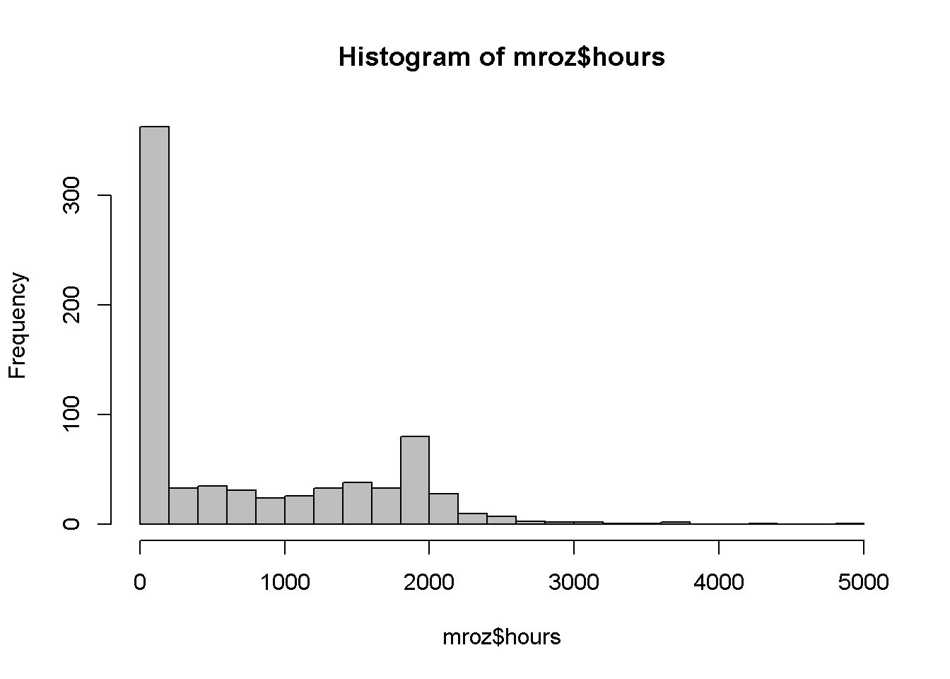
Figure 16.2: Histogram for the variable ‘wage’ in the ‘mroz’ dataset
A censored model is based on the idea of a latent, or unobserved variable that is not censored, and is explained via a probit model, as shown in Equation \ref{eq:latentVariable}.
\[\begin{equation} y_{i}^* =\beta_{1}+\beta_{2}x_{i}+e_{i} \label{eq:latentVariable} \end{equation}\]The observable variable, \(y\), is zero for all \(y^*\) that are less or equal to zero and is equal to \(y^*\) when \(y^*\) is greater than zero. The model for censored data is called Tobit, and is described by Equation \ref{eq:Tobit16}.
\[\begin{equation} P(y=0)=P(y*\leq 0)=1-\Phi [(\beta1+\beta_{2}x)/\sigma] \label{eq:Tobit16} \end{equation}\]The marginal effect of a change in \(x\) on the observed variable \(y\) is given by Equation \ref{eq:MargEffectTobit16}.
\[\begin{equation} \frac{\partial E(y | x)}{\partial x}=\beta_{2}\Phi\left( \frac{\beta_{1}+\beta_{2}x}{\sigma}\right) \label{eq:MargEffectTobit16} \end{equation}\]library(AER)
mroz.tobit <- tobit(hours~educ+exper+age+kidsl6,
data=mroz)
sMrozTobit <- summary(mroz.tobit)
sMrozTobit##
## Call:
## tobit(formula = hours ~ educ + exper + age + kidsl6, data = mroz)
##
## Observations:
## Total Left-censored Uncensored Right-censored
## 753 325 428 0
##
## Coefficients:
## Estimate Std. Error z value Pr(>|z|)
## (Intercept) 1349.8763 386.2991 3.49 0.00048 ***
## educ 73.2910 20.4746 3.58 0.00034 ***
## exper 80.5353 6.2878 12.81 < 2e-16 ***
## age -60.7678 6.8882 -8.82 < 2e-16 ***
## kidsl6 -918.9181 111.6607 -8.23 < 2e-16 ***
## Log(scale) 7.0332 0.0371 189.57 < 2e-16 ***
## ---
## Signif. codes: 0 '***' 0.001 '**' 0.01 '*' 0.05 '.' 0.1 ' ' 1
##
## Scale: 1134
##
## Gaussian distribution
## Number of Newton-Raphson Iterations: 4
## Log-likelihood: -3.83e+03 on 6 Df
## Wald-statistic: 243 on 4 Df, p-value: < 2.2e-16The following code lines calculate the marginal effect of education on hours for some given values of the regressors.
xEduc <- 12.29
xExper <- 10.63
xAge <- 42.54
xKids <- 1
bInt <- coef(mroz.tobit)[[1]]
bEduc <- coef(mroz.tobit)[[2]]
bExper <- coef(mroz.tobit)[[3]]
bAge <- coef(mroz.tobit)[[4]]
bKids <- coef(mroz.tobit)[[5]]
bSigma <- mroz.tobit$scale
Phactor <- pnorm((bInt+bEduc*xEduc+bExper*xExper+
            bAge*xAge+bKids*xKids)/bSigma)
DhoursDeduc <- bEduc*Phactor
The calculated marginal effect is \(26.606\). (The function censReg() from package censReg can also be used for estimating Tobit models; this function gives the possibility of calculating marginal effects using the function margEff().)
16.10 The Heckit, or Sample Selection Model
The models are useful when the sample selection is not random, but whehter an individual is in the sample depends on individual characteristics. For example, when studying wage determination for married women, some women are not in the labour force, therefore their wages are zero.
The model to use in such situation is Heckit, which involves two equations: the selection equation, given in Equation \ref{eq:HeckitSel16}, and the linear equation of interest, as in Equation \ref{eq:HeckitEqInterest16}.
\[\begin{equation} z_{i}^*=\gamma_{1}+\gamma_{2}w_{i}+u_{i} \label{eq:HeckitSel16} \end{equation}\] \[\begin{equation} y_{i}=\beta_{1}+\beta_{2}x_{i}+e_{i} \label{eq:HeckitEqInterest16} \end{equation}\]Estimates of the \(\beta\)s can be obtained by using least squares on the model in Equation \ref{eq:HeckitLambdaEq}, where \(\lambda_{i}\) is calculated using the formula in Equation \ref{eq:HeckitLambdaDef16}.
\[\begin{equation} y_{i}=\beta_{1}+\beta_{2}x_{i}+\beta_{\lambda}\lambda _{i}+\nu_{i} \label{eq:HeckitLambdaEq} \end{equation}\] \[\begin{equation} \lambda_{i}=\frac{\phi(\gamma_{1}+\gamma_{2}w_{i})}{\Phi(\gamma_{1}+\gamma_{2}w_{i})} \label{eq:HeckitLambdaDef16} \end{equation}\]The amount \(\lambda\) given by Equation \ref{eq:HeckitLambdaDef16} is called the inverse Mills ratio.
the Heckit procedure involves two steps, estimating both the selection equation and the equation of interest. Function selection() in the sampleSelection package performs both steps; therefore, it needs both equations among its arguments. (The selection equation is, in fact, a probit model.)
library(sampleSelection)
wage.heckit <- selection(lfp~age+educ+I(kids618+kidsl6)+mtr,
                         log(wage)~educ+exper,
                         data=mroz, method="ml")
summary(wage.heckit)
## --------------------------------------------
## Tobit 2 model (sample selection model)
## Maximum Likelihood estimation
## Newton-Raphson maximisation, 4 iterations
## Return code 2: successive function values within tolerance limit
## Log-Likelihood: -913.513
## 753 observations (325 censored and 428 observed)
## 10 free parameters (df = 743)
## Probit selection equation:
## Estimate Std. error t value Pr(> t)
## (Intercept) 1.53798 0.61889 2.49 0.013 *
## age -0.01346 0.00603 -2.23 0.026 *
## educ 0.06278 0.02180 2.88 0.004 **
## I(kids618 + kidsl6) -0.05108 0.03276 -1.56 0.119
## mtr -2.20864 0.54620 -4.04 0.000053 ***
## Outcome equation:
## Estimate Std. error t value Pr(> t)
## (Intercept) 0.64622 0.23557 2.74 0.0061 **
## educ 0.06646 0.01657 4.01 0.000061 ***
## exper 0.01197 0.00408 2.93 0.0034 **
## Error terms:
## Estimate Std. error t value Pr(> t)
## sigma 0.8411 0.0430 19.6 <2e-16 ***
## rho -0.8277 0.0391 -21.2 <2e-16 ***
## ---
## Signif. codes: 0 '***' 0.001 '**' 0.01 '*' 0.05 '.' 0.1 ' ' 1
## --------------------------------------------References
Adkins, Lee. 2014. Using Gretl for Principles of Econometrics, 4th Edition. Economics Working Paper Series. 1412. Oklahoma State University, Department of Economics; Legal Studies in Business. http://EconPapers.repec.org/RePEc:okl:wpaper:1412.