Chapter 1 Introduction
rm(list=ls()) # Caution: this clears the Environmentlibrary(bookdown)
library(PoEdata)
library(knitr)
library(xtable)
library(printr)
library(stargazer)
library(rmarkdown)Although this manual is self-contained, it can be used as a supplementary resource for the “Principles of Econometrics” textbook by Carter Hill, William Griffiths and Guay Lim, 4-th edition (Hill, Griffiths, and Lim 2011).
The following list gives some of the R packages that are used in this book more frequently:
devtools(Wickham and Chang 2016)PoEdata(Colonescu 2016)knitr(Xie 2016b)bookdown(Xie 2016a)xtable(Dahl 2016)printr(Xie 2014)stargazer(Hlavac 2015)rmarkdown(Allaire et al. 2016)
The function \(install\_git\) from the package devtools installs packages such as PoEdata from the GitHub web site. Here is the code that installs devtools and bookdown:
install.packages("devtools")
devtools::install_git(
  "https://github.com/ccolonescu/PoEdata")
The computing environment for using R (R Development Core Team 2008) is RStudio (RStudio Team 2015). You need to install on your computer the following resources:
- R (https://cloud.r-project.org/)
- RStudio (https://www.rstudio.com/products/rstudio/download/)
- PoEdata package (https://github.com/ccolonescu/PoEdata)
This brief introduction to R does not intend to be exhaustive, but to cover the minimum material used in this book. Please refer to the R documentation and to many other resuorces for additional information. For beginners, I would recommend (Lander 2013).
1.1 The RStudio Screen
A typical RStudio Screen is divided in four quadrants, as Figure 1.1 shows. The NW quadrant is for writing your script and for viewing data.
knitr::include_graphics(
  "01-intro_files/RStudio_screen_1.PNG")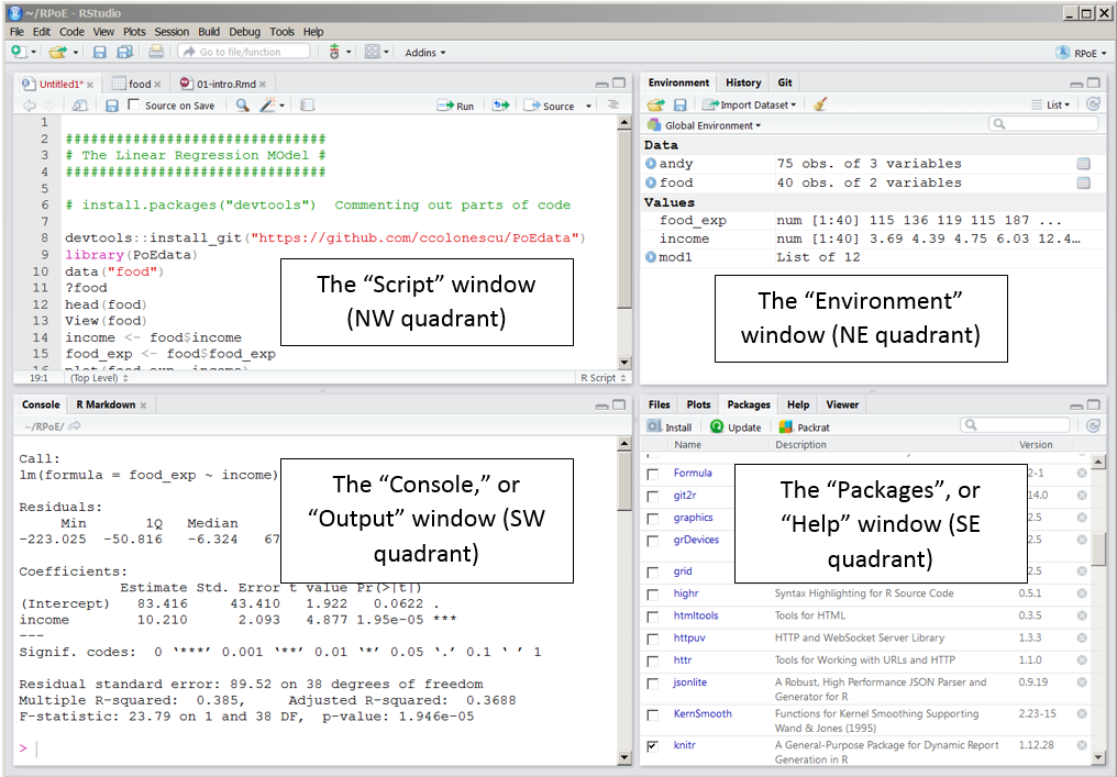
Figure 1.1: The four quadrants of an RStudio screen
1.1.1 The Script, or data view window
Here are a few tips for writing and executing script in the Script window:
- You may start your script with a comment showing a title and a brief description of what the script does. A “comment” line starts with the hash character (
#). Comments can be inserted anywhere in the script, even in line with code, but what follows the hash character to the end of the line will be disregarded by R. - Code lines may be continued on the next line with no special character to announce a line continuation. However, code will be continued on the next line only if the previous line ends in a way that requires continuation, for instance with a comma or unclosed brackets.
- When you want to run a certain line of code, place the cursor anywhere on the line and press
Ctrl+Enter; if you want to run a sequence of several code lines, select the respective sequence and pressCtrl+Enter.
1.1.2 The console, or output window
While it is always advisable to work in the script mode because it can be saved and re-used for different data, sometimes we need to run commands that are out of the script context. Such commands can be typed at the bottom of the console at the sign >. Pressing Enter executes such a command, and the up and down arrows allow re-activating and editing older lines of code that had been previously typed into the console.
1.2 How to Open a Data File
To open a data file for the Principles of Econometrics textbook, (Hill, Griffiths, and Lim 2011), first check if the devtools package is installed. If it is not, run the code install.packages("devtools") in the console.
devtools::install_git(
  "https://github.com/ccolonescu/PoEdata")
library(PoEdata) # Makes datasets ready to use
Now, we can load and inspect a particular dataset, for example “andy.” When the dataset is available, it sould show in the Environment window (look up and right).
library(PoEdata)
data("andy")  # makes the dataset "andy" ready to use
?andy         # shows information about the dataset

# Show head of dataset, with variables as column names:
head(andy)

# Show a few rows in dataset:
some(andy)
1.3 Creating Graphs
The basic tools for graph creating are the following R functions
plot(x, y, xlab="income in 100", ylab="food expenditure, in $", type="p"), wherexandystand for the variable names to be plotted,xlabandylabare the labels you wish to see on the plot, andtyperefers to the style of the plot;typecan be one of the following: “p” (points), “l” for lines, and “b” for both points and lines, “n” for no plot. The type value “n” creates an empty graph which seres other functions such asabline(), which is described below.- The function
curve()plots a curve described by a mathematical function, say \(f\), over a specified interval . When the argumentadd = TRUEis present, the fuction adds the curve to a previously plotted graph. Figure 1.2 is an example.
curve(x^1, from=-2, to=2, xlab="x", ylab="y = x" )
# Add another curve to the existing graph:
curve(x^2, add = TRUE)
#plot(1:100, type='n')
curve(sqrt(x), from=0, to=100, xlab="x", ylab="y")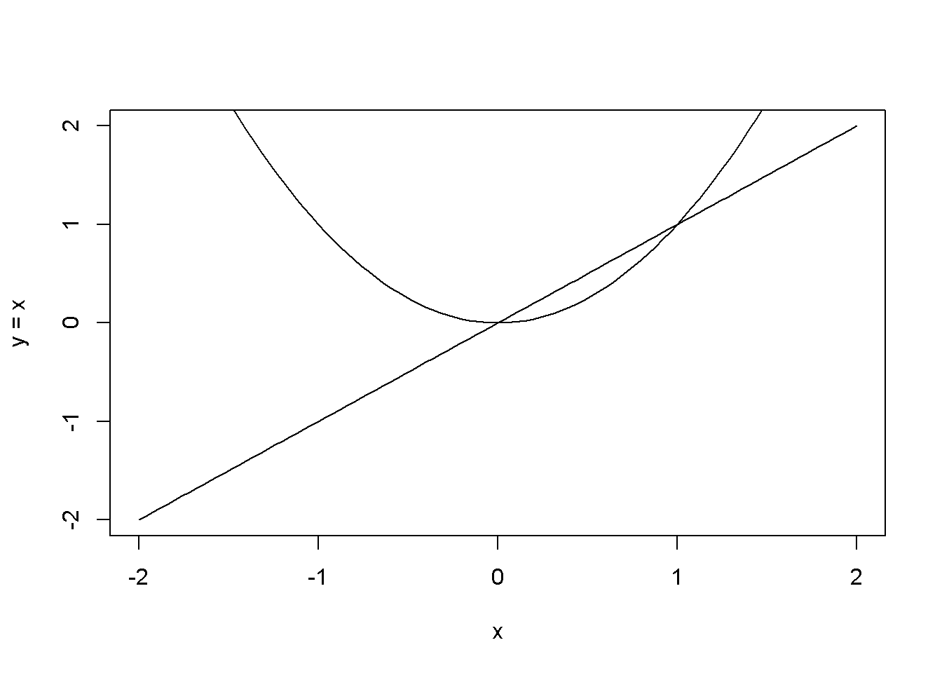
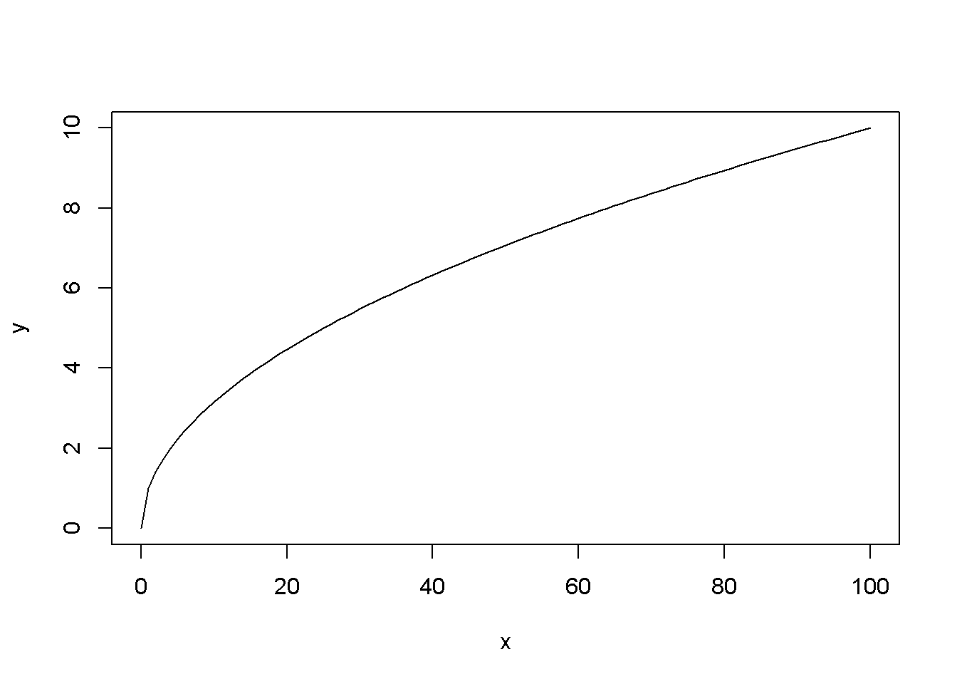
Figure 1.2: Examples of using the function curve()
- The function
abline()adds a line defined by its interceptaand slopebto the current graph. The arguments of the function are: besidesaandb, the arguments of the function are:h, the \(y\)-value for a horizontal line;v, the \(x\)-value for a vertical line;coef, the name of a simple linear regression object, which includes the intercept and slope of a regression line.
plot(1:10, type="n") # creates an empty graph
# Add straight lines to graph:
abline(a=8, b=-0.5, h=3.5, v=4)
curve(x^2, from=0, to=20)
abline(v=10)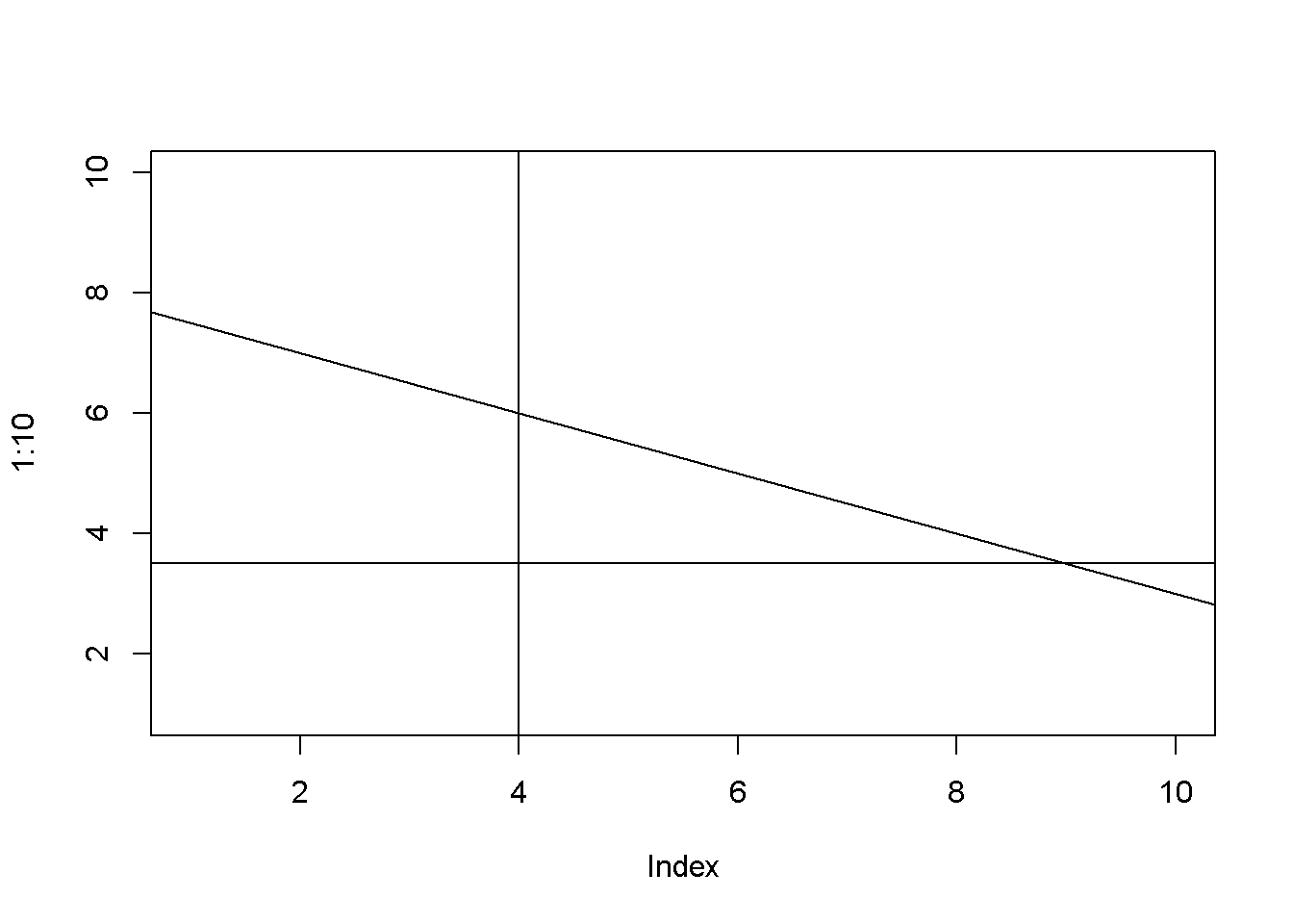
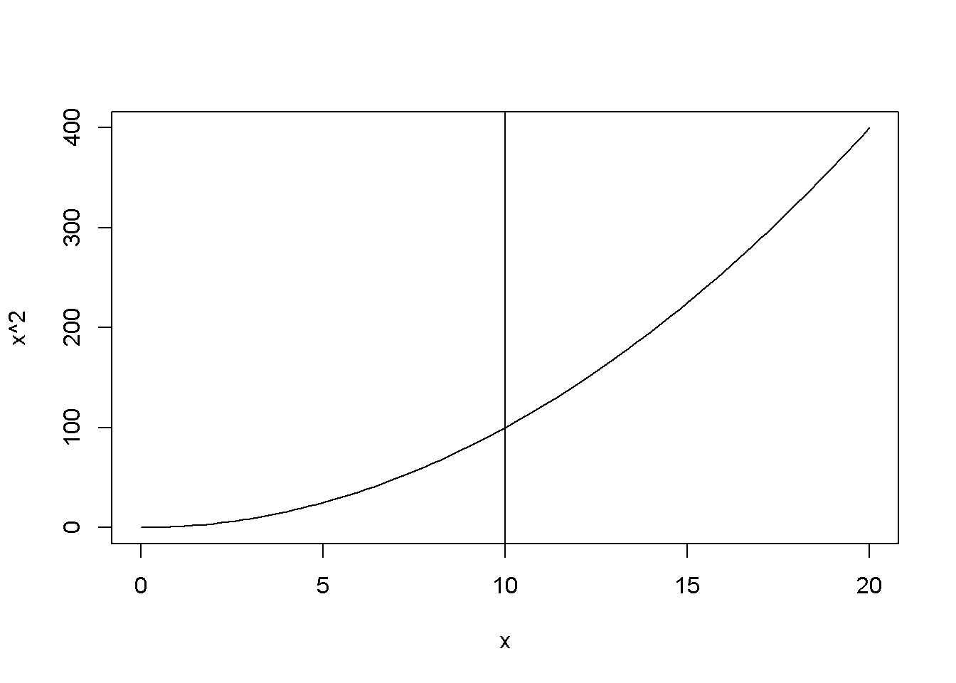
Figure 1.3: Examples of using the function abline()
1.4 An R Cheat Sheet
Here is an overview of some R commands used in this book.
lm(y~x, data = datafile) regresses y on x using the data in datafile
nrow(datafile) returns the number of observations (raws) in datafile
nobs(modelname) gives the number of observations used by a model. This may be different from the number of observation in the data file because of missing values or sub-sampling
set.seed(number) sets the seed for the random number generator to make results reproducible. This is needed to construct random subsamples of data
rm(list=ls()) removes all objects in the current Environment except those that have names starting with a dot (.)
References
Hill, R.C., W.E. Griffiths, and G.C. Lim. 2011. Principles of Econometrics. Wiley. https://books.google.ie/books?id=Q-fwbwAACAAJ.
Wickham, Hadley, and Winston Chang. 2016. Devtools: Tools to Make Developing R Packages Easier. https://CRAN.R-project.org/package=devtools.
Colonescu, Constantin. 2016. PoEdata: PoE Data for R.
Xie, Yihui. 2016b. Knitr: A General-Purpose Package for Dynamic Report Generation in R. https://CRAN.R-project.org/package=knitr.
Xie, Yihui. 2016a. Bookdown: Authoring Books with R Markdown. https://CRAN.R-project.org/package=bookdown.
Dahl, David B. 2016. Xtable: Export Tables to Latex or Html. https://CRAN.R-project.org/package=xtable.
Xie, Yihui. 2014. Printr: Automatically Print R Objects According to Knitr Output Format. http://yihui.name/printr.
Hlavac, Marek. 2015. Stargazer: Well-Formatted Regression and Summary Statistics Tables. https://CRAN.R-project.org/package=stargazer.
Allaire, JJ, Joe Cheng, Yihui Xie, Jonathan McPherson, Winston Chang, Jeff Allen, Hadley Wickham, Aron Atkins, and Rob Hyndman. 2016. Rmarkdown: Dynamic Documents for R. http://rmarkdown.rstudio.com.
R Development Core Team. 2008. R: A Language and Environment for Statistical Computing. Vienna, Austria: R Foundation for Statistical Computing. http://www.R-project.org.
RStudio Team. 2015. RStudio: Integrated Development Environment for R. Boston, MA: RStudio, Inc. http://www.rstudio.com/.
Lander, Jared P. 2013. R for Everyone: Advanced Analytics and Graphics. 1st ed. Addison-Wesley Professional.