Chapter 2 The Simple Linear Regression Model

rm(list=ls()) # Caution: this clears the Environment

2.1 The General Model

A simple linear regression model assumes that a linear relationship exists between the conditional expectation of a dependent variable, $y$, and an independent variable, $x$. Sometimes I call the independent variable ‘response’ or ‘response variable’, and the independent variables ‘regressors.’ The assumed relationship in a linear regression model has the form \[\begin{equation} y_{i}=\beta_{1}+\beta_{2}x_{i}+e_{i}, \label{eq:simplelm} \end{equation}\]

where

$y$ is the dependent variable
$x$ is the independent variable
$e$ is an error term
$\sigma^2$ is the variance of the error term
$\beta_1$ is the intercept parameter or coefficient
$\beta_2$ is the slope parameter or coefficient
$i$ stands fot the i -th observation in the dataset, $i=1,2, ...,N$
$N$ is the number of observations in the dataset

The predicted, or estimated value of $y$ given $x$ is given by Equation \ref{eq:pred1}; in general, the hat symbol indicates an estimated or a predicted value.

\[\begin{equation} \hat{y} = b_{1} + b_{2} x \label{eq:pred1} \end{equation}\]

The simple linear regression model assumes that the values of $x$ are previously chosen (therefore, they are non-random), that the variance of the error term, $\sigma^2$, is the same for all values of $x$, and that there is no connection between one observation and another (no correlation between the error terms of two observations). In addition, it is assumed that the expected value of the error term for any value of $x$ is zero.

The subscript $i$ in Equation \ref{eq:simplelm} indicates that the relationship applies to each of the $N$ observations. Thus, there must be specific values of $y$, $x$, and $e$ for each observation. However, since $x$ is not random, there are, typically, several observations sharing the same $x$, as the scatter diagram in Figure 2.1 shows.

library(PoEdata)
data("cps_small")
plot(cps_small$educ, cps_small$wage, 
     xlab="education", ylab="wage")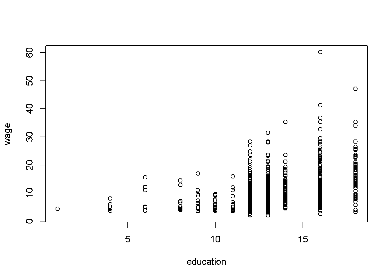

Figure 2.1: Example of several observations for any given $x$

2.2 Example: Food Expenditure versus Income

The data for this example is stored in the R package PoEdata (To check if the package PoEdata is installed, look in the Packages list.)

library(PoEdata)
data(food)
head(food)

food_exp	income
115.22	3.69
135.98	4.39
119.34	4.75
114.96	6.03
187.05	12.47
243.92	12.98

It is always a good idea to visually inspect the data in a scatter diagram, which can be created using the function plot(). Figure 2.2 is a scatter diagram of food expenditure on income, suggesting that there is a positive relationship between income and food expenditure.

data("food", package="PoEdata")
plot(food$income, food$food_exp, 
     ylim=c(0, max(food$food_exp)),
     xlim=c(0, max(food$income)),
     xlab="weekly income in $100", 
     ylab="weekly food expenditure in $", 
     type = "p")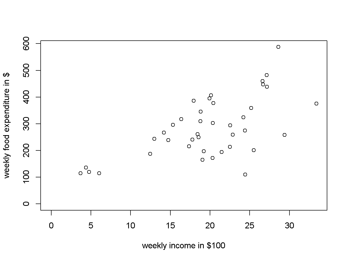

Figure 2.2: A scatter diagram for the food expenditure model

2.3 Estimating a Linear Regression

The R function for estimating a linear regression model is lm(y~x, data) which, used just by itself does not show any output; It is useful to give the model a name, such as mod1, then show the results using summary(mod1). If you are interested in only some of the results of the regression, such as the estimated coefficients, you can retrieve them using specific functions, such as the function coef(). For the food expenditure data, the regression model will be

\[\begin{equation} food\_exp = \beta_{1} + \beta_{2} income + e \label{eq:foodexpeq} \end{equation}\]

where the subscript $i$ has been omitted for simplicity.

library(PoEdata)
mod1 <- lm(food_exp ~ income, data = food)
b1 <- coef(mod1)[[1]]
b2 <- coef(mod1)[[2]]
smod1 <- summary(mod1)
smod1

## 
## Call:
## lm(formula = food_exp ~ income, data = food)
## 
## Residuals:
##     Min      1Q  Median      3Q     Max 
## -223.03  -50.82   -6.32   67.88  212.04 
## 
## Coefficients:
##             Estimate Std. Error t value Pr(>|t|)    
## (Intercept)    83.42      43.41    1.92    0.062 .  
## income         10.21       2.09    4.88 0.000019 ***
## ---
## Signif. codes:  0 '***' 0.001 '**' 0.01 '*' 0.05 '.' 0.1 ' ' 1
## 
## Residual standard error: 89.5 on 38 degrees of freedom
## Multiple R-squared:  0.385,  Adjusted R-squared:  0.369 
## F-statistic: 23.8 on 1 and 38 DF,  p-value: 0.0000195

The function coef() returns a list containing the estimated coefficients, where a specific coefficient can be accessed by its position in the list. For example, the estimated value of $\beta_1$ is b1 <- coef(mod1)[[1]], which is equal to 83.416002, and the estimated value of $\beta_2$ is b2 <- coef(mod1)[[2]], which is equal to 10.209643.

The intercept parameter, $\beta_{1}$, is usually of little importance in econometric models; we are mostly interested in the slope parameter, $\beta_{2}.$ The estimated value of $\beta_2$ suggests that the food expenditure for an average family increases by 10.209643 when the family income increases by 1 unit, which in this case is $100. The $R$ function abline() adds the regfression line to the prevoiusly plotted scatter diagram, as Figure 2.3 shows.

plot(food$income, food$food_exp, 
     xlab="weekly income in $100", 
     ylab="weekly food expenditure in $", 
     type = "p")
abline(b1,b2)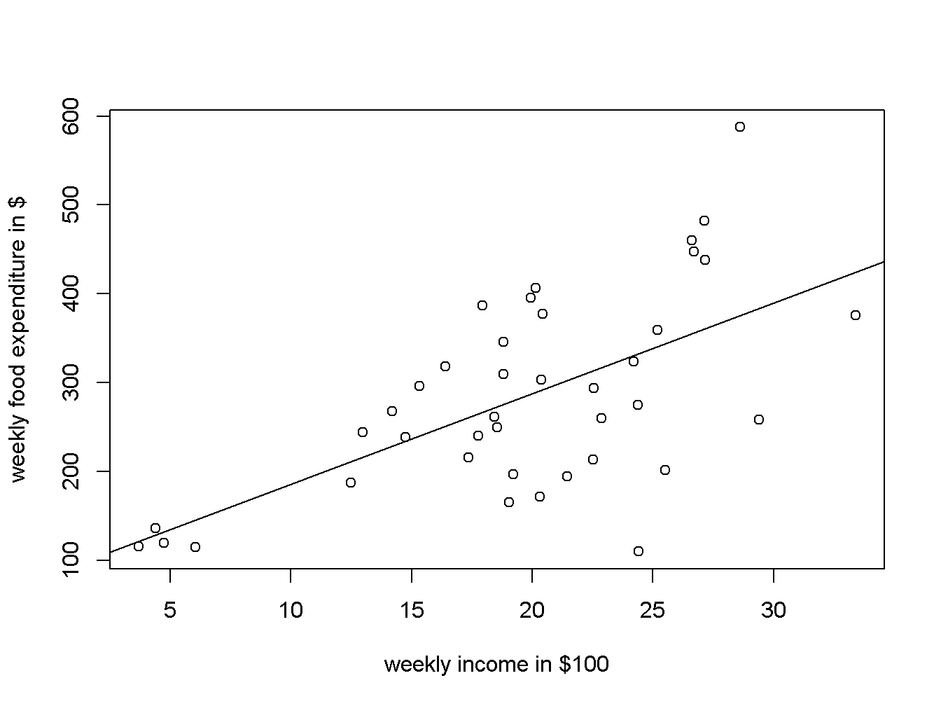

Figure 2.3: Scatter diagram and regression line for the food expenditure model

How can one retrieve various regression results? These results exist in two R objects produced by the lm() function: the regression object, such as mod1 in the above code sequence, and the regression summary, which I denoted by smod1. The next code shows how to list the names of all results in each object.

names(mod1)

##  [1] "coefficients"  "residuals"     "effects"       "rank"         
##  [5] "fitted.values" "assign"        "qr"            "df.residual"  
##  [9] "xlevels"       "call"          "terms"         "model"

names(smod1)

##  [1] "call"          "terms"         "residuals"     "coefficients" 
##  [5] "aliased"       "sigma"         "df"            "r.squared"    
##  [9] "adj.r.squared" "fstatistic"    "cov.unscaled"

To retrieve a particular result you just refer to it with the name of the object, followed by the $ sign and the name of the result you wish to retrieve. For instance, if we want the vector of coefficients from mod1, we refer to it as mod1$coefficients and smod1$coefficients:

mod1$coefficients

## (Intercept)      income 
##     83.4160     10.2096

smod1$coefficients

	Estimate	Std. Error	t value	Pr(>\|t\|)
(Intercept)	83.4160	43.41016	1.92158	0.062182
income	10.2096	2.09326	4.87738	0.000019

As we have seen before, however, some of these results can be retrieved using specific functions, such as coef(mod1), resid(mod1), fitted(mod1), and vcov(mod1).

2.4 Prediction with the Linear Regression Model

The estimated regression parameters, $b_{1}$ and $b_{2}$ allow us to predict the expected food expenditure for any given income. All we need to do is to plug the estimated parameter values and the given income into an equation like Equation \ref{eq:pred1}. For example, the expected value of $food\_exp$ for an income of $2000 is calculated in Equation \ref{eq:pred2}. (Remember to divide the income by 100, since the data for the variable $income$ is in hundreds of dollars.)

\[\begin{equation} \widehat{food\_ exp} = 83.416002 + 10.209643 * 20 = \$ 287.608861 \label{eq:pred2} \end{equation}\]

R, however, does this calculations for us with its function called predict(). Let us extend slightly the example to more than one income for which we predict food expenditure, say income = $2000, $2500, and $2700. The function predict() in R requires that the new values of the independent variables be organized under a particular form, called a data frame. Even when we only want to predict for one income, we need the same data-frame structure. In R, a set of numbers is held together using the structure c(). The following sequence shows this example.

# library(PoEdata) (load the data package if you have not done so yet)
mod1 <- lm(food_exp~income, data=food)
newx <- data.frame(income = c(20, 25, 27))
yhat <- predict(mod1, newx)
names(yhat) <- c("income=$2000", "$2500", "$2700") 
yhat  # prints the result

## income=$2000        $2500        $2700 
##      287.609      338.657      359.076

2.5 Repeated Samples to Assess Regression Coefficients

The regression coefficients $b_{1}$ and $b_{2}$ are random variables, because they depend on sample. Let us construct a number of random subsamples from the food data and re-calculate $b_{1}$ and $b_{2}$. A random subsample can be constructed using the function sample(), as the following example illustrates only for $b_{2}$.

N <- nrow(food) # returns the number of observations in the dataset
C <- 50         # desired number of subsamples
S <- 38         # desired sample size

sumb2 <- 0
for (i in 1:C){   # a loop over the number of subsamples
  set.seed(3*i)   # a different seed for each subsample  
  subsample <- food[sample(1:N, size=S, replace=TRUE), ]
  mod2 <- lm(food_exp~income, data=subsample)
  #sum b2 for all subsamples:
  sumb2 <- sumb2 + coef(mod2)[[2]]
}
print(sumb2/C, digits = 3)

## [1] 9.88

The result, $b_{2}=$ 9.88, is the average of 50 estimates of $b_{2}$.

2.6 Estimated Variances and Covariance of Regression Coefficients

Many applications require estimates of the variances and covariances of the regression coefficients. R stores them in the a matrix vcov():

(varb1 <- vcov(mod1)[1, 1])

## [1] 1884.44

(varb2 <- vcov(mod1)[2, 2])

## [1] 4.38175

(covb1b2 <- vcov(mod1)[1,2])

## [1] -85.9032

2.7 Non-Linear Relationships

Sometimes the scatter plot diagram or some theoretical consideraions suggest a non-linear relationship. The most popular non-linear relationships involve logarithms of the dependent or independent variables and polinomial functions.

The quadratic model requires the square of the independent variable.

\[\begin{equation} y_{i}=\beta_{1}+\beta_{2}x_{i}^2+e_{i} \label{eq:quadratic2} \end{equation}\]

In R, independent variables involving mathematical operators can be included in a regression equation with the function I(). The following example uses the dataset br from the package PoEdata, which includes the sale prices and the attributes of 1080 houses in Baton Rouge, LA. price is the sale price in dollars, and sqft is the surface area in square feet.

library(PoEdata)
data(br)
mod3 <- lm(price~I(sqft^2), data=br)
b1 <- coef(mod3)[[1]]
b2 <- coef(mod3)[[2]]
sqftx=c(2000, 4000, 6000) #given values for sqft
pricex=b1+b2*sqftx^2 #prices corresponding to given sqft 
DpriceDsqft <- 2*b2*sqftx # marginal effect of sqft on price
elasticity=DpriceDsqft*sqftx/pricex 
b1; b2; DpriceDsqft; elasticity #prints results

## [1] 55776.6

## [1] 0.0154213

## [1]  61.6852 123.3704 185.0556

## [1] 1.05030 1.63125 1.81741

We woud like now to draw a scatter diagram and see how the quadratic function fits the data. The next chunk of code provides two alternatives for constructing such a graph. The first simply draws the quadratic function on the scatter diagram, using the R function curve(); the second uses the function lines, which requires ordering the dataset in increasing values of sqft before the regression model is evaluated, such that the resulting fitted values will also come out in the same order.

mod31 <- lm(price~I(sqft^2), data=br)
plot(br$sqft, br$price, xlab="Total square feet", 
     ylab="Sale price, $", col="grey")
#add the quadratic curve to the scatter plot:
curve(b1+b2*x^2, col="red", add=TRUE)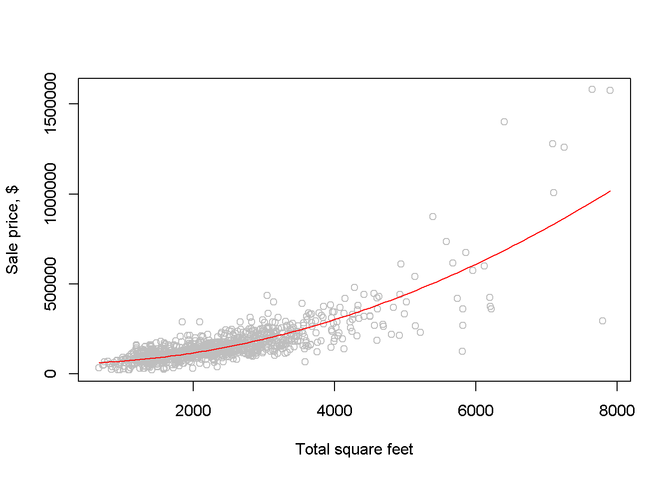

Figure 2.4: Fitting a quadratic model to the br dataset

An alternative way to draw the fitted curve:

ordat <- br[order(br$sqft), ] #sorts the dataset after `sqft`
mod31 <- lm(price~I(sqft^2), data=ordat)
plot(br$sqft, br$price, 
     main="Dataset ordered after 'sqft' ", 
     xlab="Total square feet", 
     ylab="Sale price, $", col="grey")
lines(fitted(mod31)~ordat$sqft, col="red")

The log-linear model regresses the log of the dependent variable on a linear expression of the independent variable (unless otherwise specified, the log notation stands for natural logarithm, following a usual convention in economics):

\[\begin{equation} log(y_{i})=\beta_{1}+\beta_{2}x_{i}+e_{i} \label{eq:loglin2} \end{equation}\]

One of the reasons to use the log of an independent variable is to make its distribution closer to the normal distribution. Let us draw the histograms of price and log(price) to compare them (see Figure 2.5). It can be noticed that that the log is closer to the normal distribution.

hist(br$price, col='grey')
hist(log(br$price), col='grey')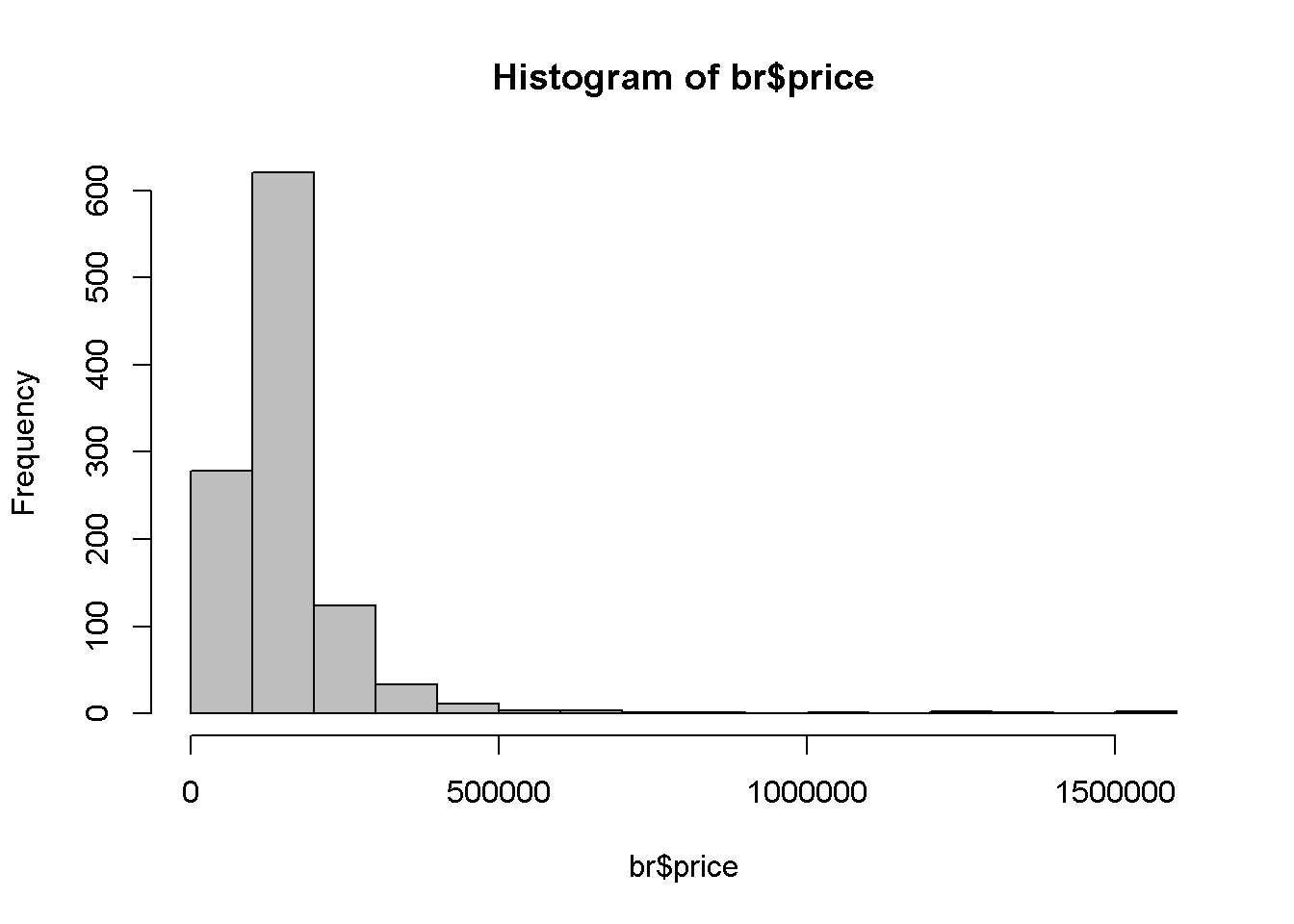

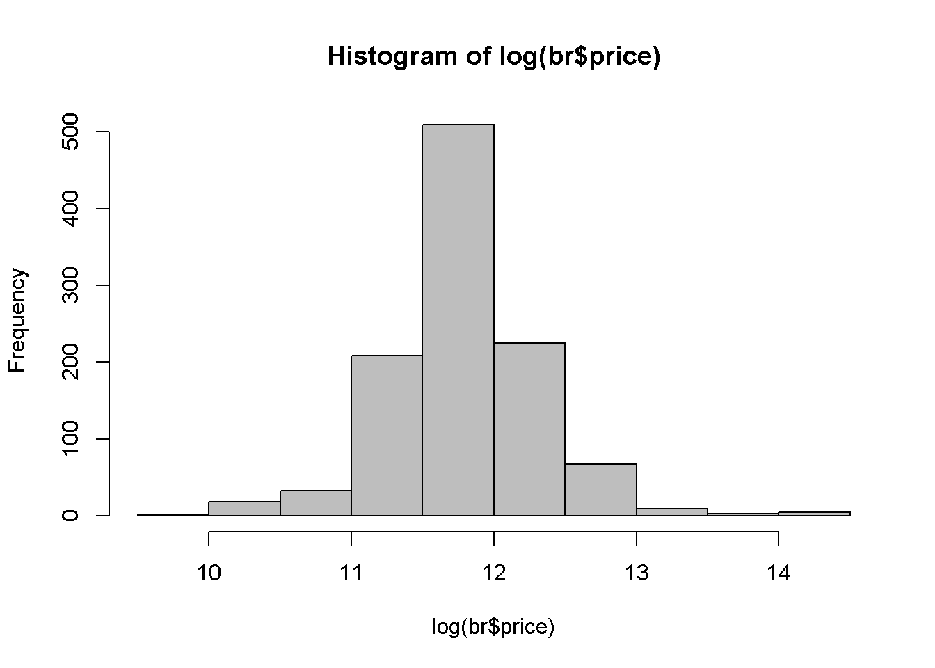
Figure 2.5: A comparison between the histograms of price and log(price)

We are interested, as before, in the estimates of the coefficients and their interpretation, in the fitted values of price, and in the marginal effect of an increase in sqft on price.

library(PoEdata)
data("br")
mod4 <- lm(log(price)~sqft, data=br)

The coefficients are $b_{1}=$ $10.84$ and $b_{2}=$ $0.00041$, showing that an increase in the surface area (sqft) of an apartment by one unit (1 sqft) increases the price of the apartment by $0.041$ percent. Thus, for a house price of $100,000, an increase of 100 sqft will increase the price by approximately $100* 0.041$ percent, which is equal to $4112.7. In general, the marginal effect of an increase in $x$ on $y$ in Equation \ref{eq:loglin2} is

\[\begin{equation} \frac{dy}{dx}=\beta_{2}y, \label{eq:loglin2margeffect} \end{equation}\]

and the elasticity is

\[\begin{equation} \epsilon =\frac{dy}{dx} \frac{x}{y} = \beta_{2}x. \label{eq:loglin2elast} \end{equation}\]

The next lines of code show how to draw the fitted values curve of the loglinear model and how to calculate the marginal effect and the elasticity for the median price in the dataset. The fitted values are here calculated using the formula

\[\begin{equation} \hat{y} = e^{b_{1}+b_{2}x} \label{loglinyhat} \end{equation}\]

ordat <- br[order(br$sqft), ] #order the dataset
mod4 <- lm(log(price)~sqft, data=ordat)
plot(br$sqft, br$price, col="grey")
lines(exp(fitted(mod4))~ordat$sqft, 
      col="blue", main="Log-linear Model")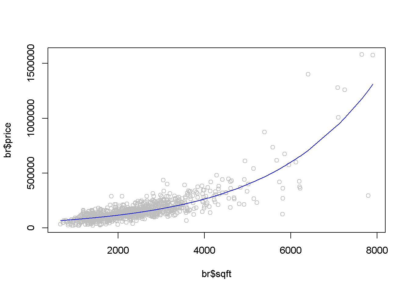

Figure 2.6: The fitted value curve in the log-linear model

pricex<- median(br$price)
sqftx <- (log(pricex)-coef(mod4)[[1]])/coef(mod4)[[2]]
(DyDx <- pricex*coef(mod4)[[2]])

## [1] 53.465

(elasticity <- sqftx*coef(mod4)[[2]])

## [1] 0.936693

R allows us to calculate the same quantities for several (sqft, price) pairs at a time, as shown in the following sequence:

b1 <- coef(mod4)[[1]]
b2 <- coef(mod4)[[2]]
#pick a few values for sqft:
sqftx <- c(2000, 3000, 4000) 
#estimate prices for those and add one more:
pricex <- c(100000, exp(b1+b2*sqftx)) 
#re-calculate sqft for all prices:
sqftx <- (log(pricex)-b1)/b2 
#calculate and print elasticities:
(elasticities <- b2*sqftx)

## [1] 0.674329 0.822538 1.233807 1.645075

2.8 Using Indicator Variables in a Regression

An indicator, or binary variable marks the presence or the absence of some attribute of the observational unit, such as gender or race if the observational unit is an individual, or location if the observational unit is a house. In the dataset utown, the variable utown is $1$ if a house is close to the university and $0$ otherwise. Here is a simple linear regression model that involves the variable utown:

\[\begin{equation} price_{i}=\beta_{1}+\beta_{2}utown_{i} \label{eq:utown} \end{equation}\]

The coefficient of such a variable in a simple linear model is equal to the difference between the average prices of the two categories; the intercept coefficient of the model in Equation \ref{eq:utown} is equal to the average price of the houses that are not close to university. Let us first calculate the average prices for each category, wich are denoted in the following sequence of code price0bar and price1bar:

data(utown)
price0bar <- mean(utown$price[which(utown$utown==0)])
price1bar <- mean(utown$price[which(utown$utown==1)])

The results are: $\overline{price}=277.24$ close to university, and $\overline{price}=215.73$ for those not close. I now show that the same results yield the coefficients of the regression model in Equation \ref{eq:utown}:

mod5 <- lm(price~utown, data=utown)
b1 <- coef(mod5)[[1]] 
b2 <- coef(mod5)[[2]]

The results are: $\overline{price}=b_{1}=215.73$ for non-university houses, and $\overline{price}=b_{1}+b_{2}=277.24$ for university houses.

2.9 Monte Carlo Simulation

A Monte Carlo simulation generates random values for the dependent variable when the regression coefficients and the distribution of the random term are given. The following example seeks to determine the distribution of the independent variable in the food expenditure model in Equation \ref{eq:foodexpeq}.

N <- 40
x1 <- 10
x2 <- 20
b1 <- 100
b2 <- 10
mu <- 0
sig2e <- 2500
sde <- sqrt(sig2e)
yhat1 <- b1+b2*x1
yhat2 <- b1+b2*x2
curve(dnorm(x, mean=yhat1, sd=sde), 0, 500, col="blue")
curve(dnorm(x, yhat2, sde), 0,500, add=TRUE, col="red")
abline(v=yhat1, col="blue", lty=2)
abline(v=yhat2, col="red", lty=2)
legend("topright", legend=c("f(y|x=10)", 
                            "f(y|x=20)"), lty=1,
       col=c("blue", "red"))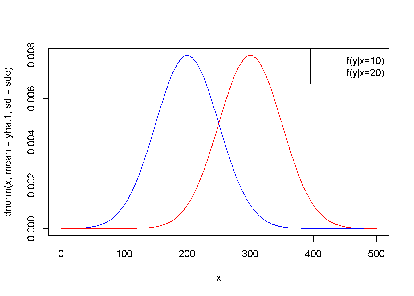

Figure 2.7: The theoretical (true) probability distributions of food expenditure, given two levels of income

Next, we calculate the variance of $b_{2}$ and plot the corresponding density function. \[\begin{equation} var(b_{2})=\frac{\sigma ^{2}}{\sum(x_{i}-\bar{x})} \label{eq:varb22} \end{equation}\]

x <- c(rep(x1, N/2), rep(x2,N/2))
xbar <- mean(x)
sumx2 <- sum((x-xbar)^2)
varb2 <- sig2e/sumx2
sdb2 <- sqrt(varb2)
leftlim <- b2-3*sdb2
rightlim <- b2+3*sdb2
curve(dnorm(x, mean=b2, sd=sdb2), leftlim, rightlim)
abline(v=b2, lty=2)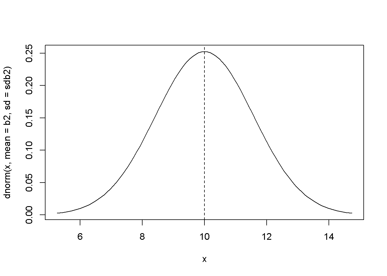

$The theoretical (true) probability density function of $b_{2}$$

Figure 2.8: The theoretical (true) probability density function of $b_{2}$

Now, with the same values of $b_{1}$, $b_{2}$, and error standard deviation, we can generate a set of values for $y$, regress $y$ on $x$, and calculate an estimated values for the coefficient $b_{2}$ and its standard error.

set.seed(12345)
y <- b1+b2*x+rnorm(N, mean=0, sd=sde)
mod6 <- lm(y~x)
b1hat <- coef(mod6)[[1]]
b2hat <- coef(mod6)[[2]]
mod6summary <- summary(mod6) #the summary contains the standard errors
seb2hat <- coef(mod6summary)[2,2]

The results are $b_{2}=$ 11.64 and $se(b_{2})=$ 1.64. The strength of a Monte Carlo simulation is, however, the possibility of repeating the estimation of the regression parameters for a large number of automatically generated samples. Thus, we can obtain a large number of values for a parameter, say $b_{2}$, and then determine its sampling characteristics. For instance, if the mean of these values is close to the initially asumed value $b_{2}=$ 10, we conclude that our estimator (the method of estimating the parameter) is unbiased.

We are going to use this time the values of $x$ in the food dataset, and generate $y$ using the linear model with $b_{1}=$ 100 and $b_{2}=$ 10.

data("food")
N <- 40
sde <- 50
x <- food$income
nrsim <- 1000
b1 <- 100
b2 <- 10
vb2 <- numeric(nrsim) #stores the estimates of b2
for (i in 1:nrsim){
  set.seed(12345+10*i)
  y <- b1+b2*x+rnorm(N, mean=0, sd=sde)
  mod7 <- lm(y~x)
  vb2[i] <- coef(mod7)[[2]]
}
mb2 <- mean(vb2)
seb2 <- sd(vb2)

The mean and standard deviation of the estimated 40 values of $b_{2}$ are, respectively, 9.974985 and 1.152632. Figure 2.9 shows the simulated distribution of $b_{2}$ and the theoretical one.

plot(density(vb2))
curve(dnorm(x, mb2, seb2), col="red", add=TRUE)
legend("topright", legend=c("true", "simulated"), 
       lty=1, col=c("red", "black"))
hist(vb2, prob=TRUE, ylim=c(0,.4))
curve(dnorm(x, mean=mb2, sd=seb2), col="red", add=TRUE)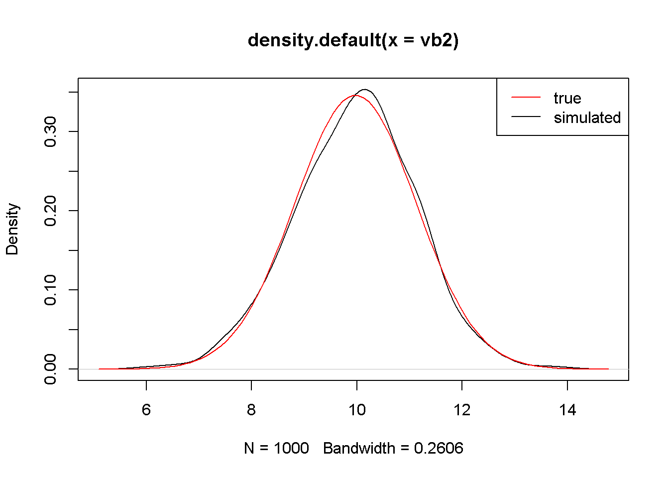

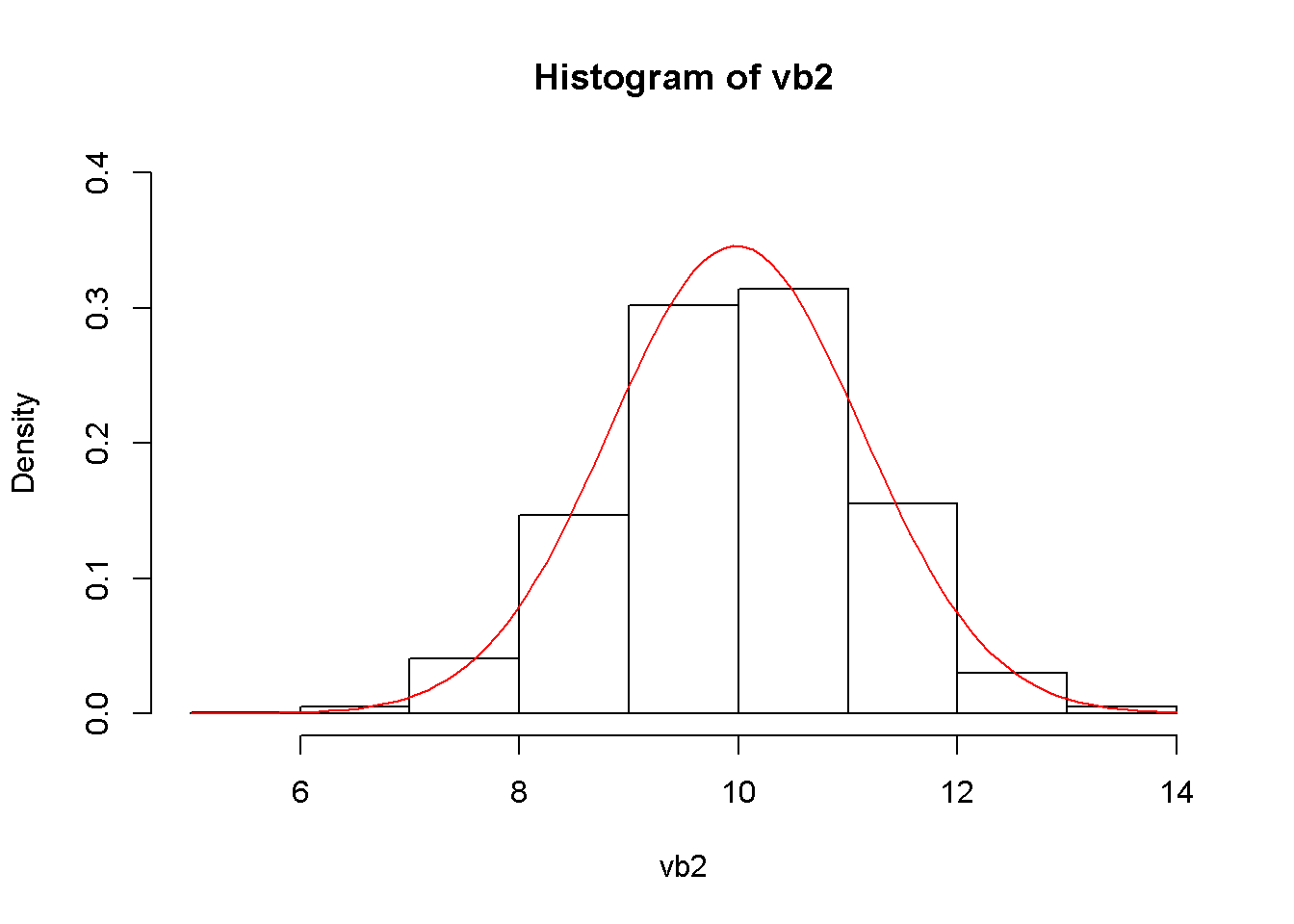
$The simulated and theoretical distributions of $b_{2}$$ $The simulated and theoretical distributions of $b_{2}$$

Figure 2.9: The simulated and theoretical distributions of $b_{2}$

rm(list=ls()) # Caution: this clears the Environment