Chapter 9 Time-Series: Stationary Variables
rm(list=ls()) #Removes all items in Environment!
library(dynlm) #for the `dynlm()` function
library(orcutt) # for the `cochrane.orcutt()` function
library(nlWaldTest) # for the `nlWaldtest()` function
library(zoo) # for time series functions (not much used here)
library(pdfetch) # for retrieving data (just mentioned here)
library(lmtest) #for `coeftest()` and `bptest()`.
library(broom) #for `glance(`) and `tidy()`
library(PoEdata) #for PoE4 datasets
library(car) #for `hccm()` robust standard errors
library(sandwich)
library(knitr) #for kable()
library(forecast)
New packages: dynlm (Zeileis 2016); orcutt (Spada, Quartagno, and Tamburini 2012); nlWaldTest (Komashko 2016); zoo [R-zoo]; pdfetch (Reinhart 2015); and forecast (Hyndman 2016).
Time series are data on several variables on an observational unit (such as an individual, country, or firm) when observations span several periods. Correlation among subsequent observations, the importance of the natural order in the data and dynamics (past values of data influence present and future values) are features of time series that do not occur in cross-sectional data.
Time series models assume, in addition to the usual linear regression assumptions, that the esries is stationary, that is, the distribution of the error term, as well as the correlation between error terms a few periods apart are constant over time. Constant distribution requires, in particular, that the variable does not display a trend in its mean or variance; constant correlation implies no clustering of observations in certain periods.
9.1 An Overview of Time Series Tools in R
\(R\) creates a time series variable or dataset using the function ts(), with the following main arguments: your data file in matrix or data frame form, the start period, the end period, the frequency of the data (1 is annual, 4 is quarterly, and 12 is monthly), and the names of your column variables. Another class of time series objects is created by the function zoo() in the package zoo, which, unlike ts(), can handle irregular or high-frequency time series. Both ts and zoo classes of objects can be used by the function dynlm() in the package with the same name to solve models that include lags and other time series specific operators.
In standard \(R\), two functions are very useful when working with time series: the difference function, \(diff(y_{t})= y_{t}-y_{t-1}\), and the lag function, \(lag(y_{t})=y_{t-1}\).
The package pdfetch is a very useful tool for getting \(R\)-compatible time series data from different online sources such as the World Bank, Eurostat, European Central Bank, and Yahoo Finance. The package WDI retrieves data from the very rich World Development Indicators database, maintained by the World Bank.
9.2 Finite Distributed Lags
A finite distributed lag model (FDL) assumes a linear relationship between a dependent variable \(y\) and several lags of an independent variable \(x\). Equation \ref{eq:fdlgen9} shows a finite distributed lag model of order q. \[\begin{equation} y_{t}=\alpha+\beta_{0}x_{t}+\beta_{1}x_{t-1}+...+\beta_{q}x_{t-q}+e_{t} \label{eq:fdlgen9} \end{equation}\]The coefficient \(\beta_{s}\) is an \(s\)-period delay multiplier, and the coefficient \(\beta_{0}\), the immediate (contemporaneous) impact of a change in \(x\) on \(y\), is an impact multiplier. If \(x\) increases by one unit today, the change in \(y\) will be \(\beta_{0}+\beta_{1}+...+\beta_{s}\) after \(s\) periods; this quantity is called the \(s\)-period interim multiplier. The total multiplier is equal to the sum of all \(\beta\)s in the model.
Let us look at Okun’s law as an example of an FDL model. Okun’s law relates contemporaneous (time \(t\)) change in unemployment rate, \(DU_{t}\), to present and past levels of economic growth rate, \(G_{t-s}\).
data("okun", package="PoEdata")
library(dynlm)
check.ts <- is.ts(okun) # "is structured as time series?"
okun.ts <- ts(okun, start=c(1985,2), end=c(2009,3),frequency=4)
okun.ts.tab <- cbind(okun.ts,
                 lag(okun.ts[,2], -1),
                 diff(okun.ts[,2], lag=1),
                 lag(okun.ts[,1], -1),
                 lag(okun.ts[,1], -2),
                 lag(okun.ts[,1], -3))
kable(head(okun.ts.tab),
      caption="The `okun` dataset with differences and lags",
col.names=c("g","u","uL1","du","gL1","gL2","gL3"))| g | u | uL1 | du | gL1 | gL2 | gL3 |
|---|---|---|---|---|---|---|
| 1.4 | 7.3 | NA | NA | NA | NA | NA |
| 2.0 | 7.2 | 7.3 | -0.1 | 1.4 | NA | NA |
| 1.4 | 7.0 | 7.2 | -0.2 | 2.0 | 1.4 | NA |
| 1.5 | 7.0 | 7.0 | 0.0 | 1.4 | 2.0 | 1.4 |
| 0.9 | 7.2 | 7.0 | 0.2 | 1.5 | 1.4 | 2.0 |
| 1.5 | 7.0 | 7.2 | -0.2 | 0.9 | 1.5 | 1.4 |
Table 9.1 shows how lags and differences work. Please note how each lag uses up an observation period.
okunL3.dyn <- dynlm(d(u)~L(g, 0:3), data=okun.ts)
kable(tidy(summary(okunL3.dyn)), digits=4,
caption="The `okun` distributed lag model with three lags")| term | estimate | std.error | statistic | p.value |
|---|---|---|---|---|
| (Intercept) | 0.5810 | 0.0539 | 10.7809 | 0.0000 |
| L(g, 0:3)0 | -0.2021 | 0.0330 | -6.1204 | 0.0000 |
| L(g, 0:3)1 | -0.1645 | 0.0358 | -4.5937 | 0.0000 |
| L(g, 0:3)2 | -0.0716 | 0.0353 | -2.0268 | 0.0456 |
| L(g, 0:3)3 | 0.0033 | 0.0363 | 0.0911 | 0.9276 |
okunL2.dyn <- dynlm(d(u)~L(g, 0:2), data=okun.ts)
kable(tidy(summary(okunL2.dyn)), digits=4,
caption="The `okun` distributed lag model with two lags")| term | estimate | std.error | statistic | p.value |
|---|---|---|---|---|
| (Intercept) | 0.5836 | 0.0472 | 12.3604 | 0.0000 |
| L(g, 0:2)0 | -0.2020 | 0.0324 | -6.2385 | 0.0000 |
| L(g, 0:2)1 | -0.1653 | 0.0335 | -4.9297 | 0.0000 |
| L(g, 0:2)2 | -0.0700 | 0.0331 | -2.1152 | 0.0371 |
Tables 9.2 and 9.3 summarize the results of linear models with 3 and 2 lags respectively. Many of the output analysis functions that we have used with the lm() function, such as summary() and coeftest() are also applicable to dynlm().
glL3 <- glance(okunL3.dyn)[c("r.squared","statistic","AIC","BIC")]
glL2 <- glance(okunL2.dyn)[c("r.squared","statistic","AIC","BIC")]
tabl <- rbind(glL3, as.numeric(glL2))
kable(tabl, caption="Goodness-of-fit statistics for `okun` models")| r.squared | statistic | AIC | BIC |
|---|---|---|---|
| 0.652406 | 42.2306 | -55.4318 | -40.1085 |
| 0.653946 | 57.9515 | -58.9511 | -46.1293 |
Table 9.4 compares the two FDL models of the \(okun\) example. The first row is the model with three lags, the second is the model with two lags. All the measures in this table points to the second model (two lags) as a better specification.
A note on how these tables were created in \(R\) is of interest. Table 9.1 was created using the function cbind, which puts together several columns (vectors); table 9.4 used two functions: rbind(), which puts together two rows, and as.numeric, which extracts only the numbers from the glance object, without the names of the columns.
9.3 Serial Correlation
Serial correlation, or autocorrelation in a time series describes the correlation between two observations separated by one or several periods. Time series tend to display autocorrelation more than cross sections because of their ordered nature. Autocorrelation could be an attribute of one series, independent of the model in which this series appears. If this series is, however, an error term, its properties do depend on the model, since error series can only exist in relation to a model.
plot(okun.ts[,"g"], ylab="growth")
plot(okun.ts[,"u"], ylab="unemployment")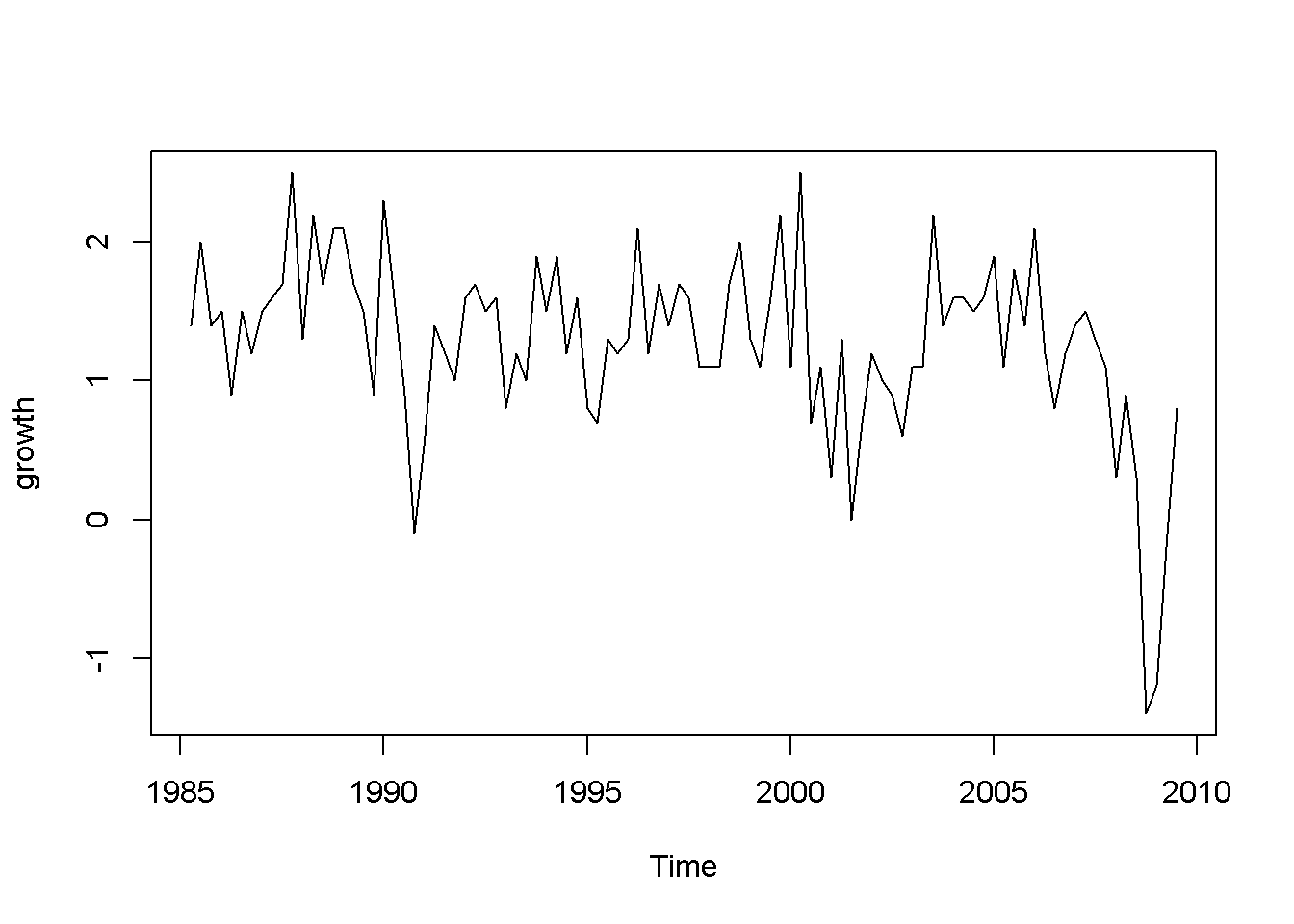
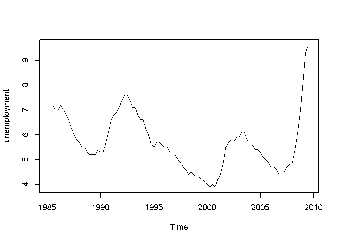
Figure 9.1: Growth and unemployment rates in the ‘okun’ dataset
The “growth” graph in Figure 9.1 display clusters of values: positive for several periods followed by a few of negative values, which is an indication of autocorrelation; the same is true for unemployment, which does not change as dramatically as growth but still shows persistence.
ggL1 <- data.frame(cbind(okun.ts[,"g"], lag(okun.ts[,"g"],-1)))
names(ggL1) <- c("g","gL1")
plot(ggL1)
meang <- mean(ggL1$g, na.rm=TRUE)
abline(v=meang, lty=2)
abline(h=mean(ggL1$gL1, na.rm=TRUE), lty=2)

ggL2 <- data.frame(cbind(okun.ts[,"g"], lag(okun.ts[,"g"],-2)))
names(ggL2) <- c("g","gL2")
plot(ggL2)
meang <- mean(ggL2$g, na.rm=TRUE)
abline(v=meang, lty=2)
abline(h=mean(ggL2$gL2, na.rm=TRUE), lty=2)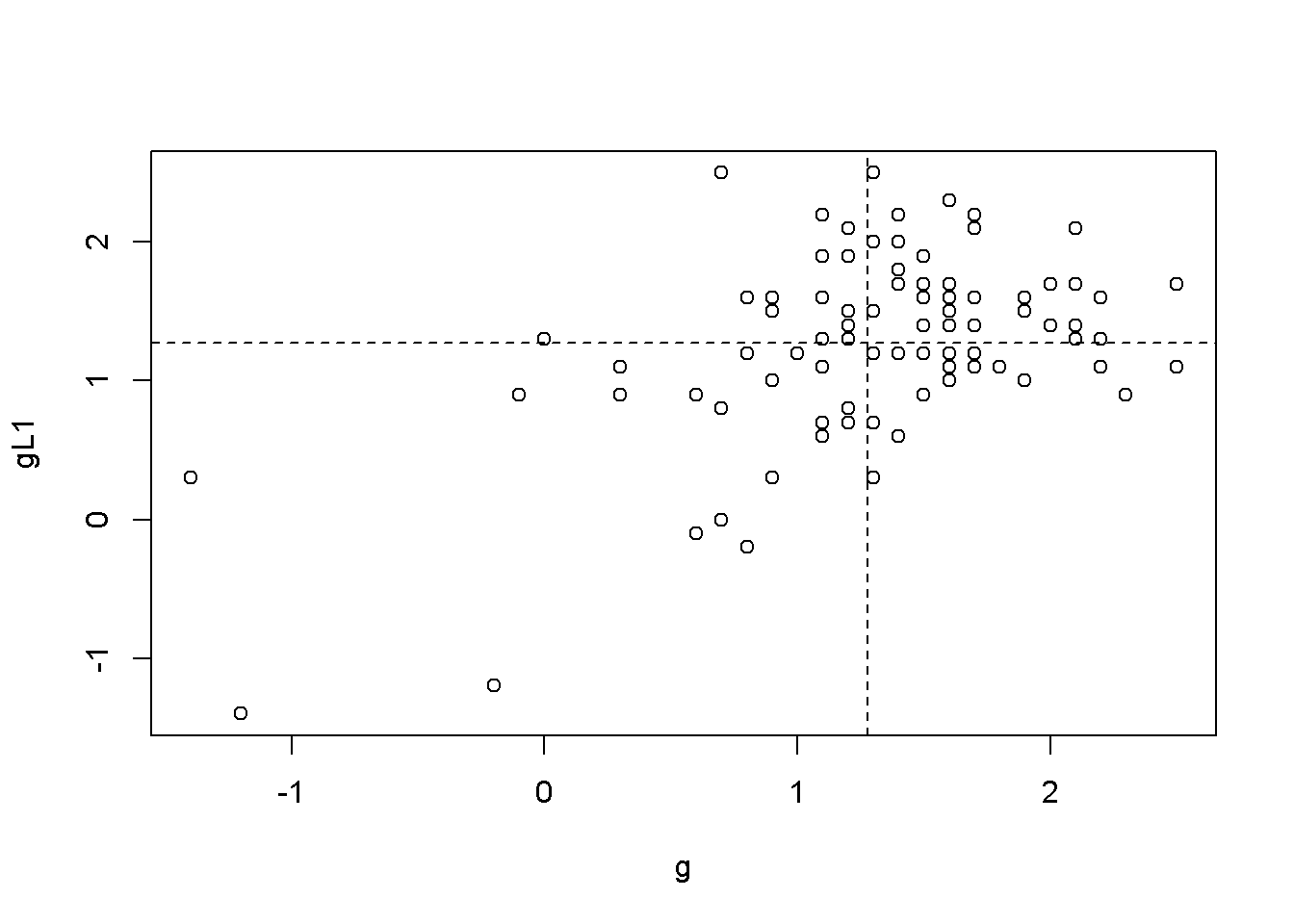
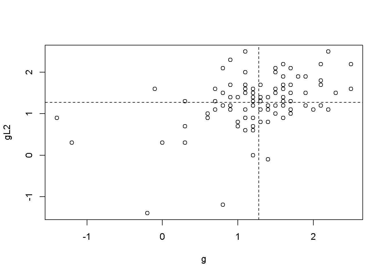
Figure 9.2: Scatter plots between ‘g’ and its lags
Figures 9.2 illustrate the correlation between the growth rate and its first two lags, which is, indeed autocorrelation. But is there a more precise test to detect autocorrelation?
Suppose we wish to test the hypothesis formulated in Equation \ref{eq:autocorhyp9}, where \(\rho_{k}\) is the population \(k\)-th order autocorrelation coefficient.
\[\begin{equation} H_{0}: \rho_{k}=0,\;\;\; H_{A}:\rho_{k}\neq 0 \label{eq:autocorhyp9} \end{equation}\] A test can be constructed based on the sample correlation coefficient, \(r_{k}\), which measures the correlation between a variable and its \(k\)-th lag; the test statistic is given in Equation \ref{eq:autocorZ9}, where \(T\) is the number of periods. \[\begin{equation} Z=\frac{r_{k}-0}{\sqrt{\frac{1}{T}}}=\sqrt{T}r_{k}\sim N(0,1) \label{eq:autocorZ9} \end{equation}\]For a \(5\%\) significance level, \(Z\) must be outside the interval \([-1.96, 1,96]\), that is, in the rejection region. Rejecting the null hypothesis is, in this case, bad news, since rejection constitutes evidence of autocorrelation. So, for a way to remember the meaning of the test, one may think of it as a test of non-autocorrelation.
The results of the (non-) autocorrelation test are usually summarized in a correlogram, a bar diagram that visualizes the values of the test statistic \(\sqrt{T}r_{k}\) for several lags as well as the \(95\%\) confidence interval. A bar (\(\sqrt{T}r_{k}\)) that exceedes (upward or downward) the limits of the confidence interval indicates autocorrelation for the corresponding lag.
growth_rate <- okun.ts[,"g"]
acf(growth_rate)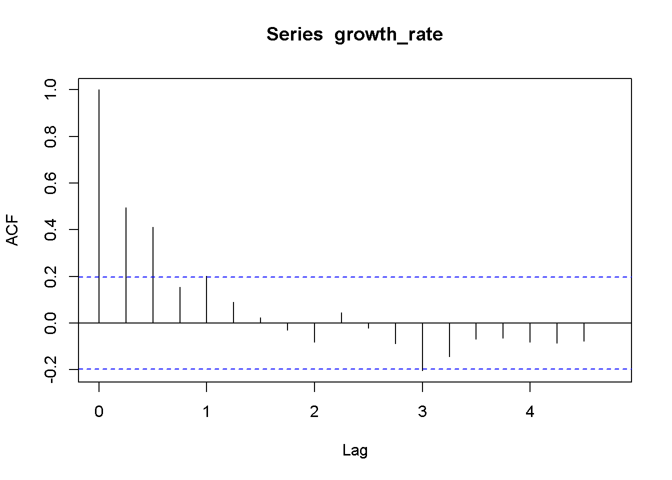
Figure 9.3: Correlogram for the growth rate, dataset ‘okun’
Figure 9.3 is a correlogram, where each bar corresponding to one lag, starting with lag 0. The correlogram shows little or no evidence of autocorrelation, except for the first and second lag (second and third bar in the figure).
Let us consider another example, the dataset phillips_aus, which containes quarterly data on unemploymnt and inflation over the period 1987Q1 to 2009Q3. We wish to apply the autocorrelation test to the error term in a time series regression to see if the non-autocorrelation in the errors is violated. Let us consider the FDL model in Equation \ref{eq:philleq9}. \[\begin{equation} inf_{t}=\beta_{1}+\beta_{2}Du_{t}+e_{t} \label{eq:philleq9} \end{equation}\]Let’s first take a look at plots of the data (visualising the data is said to be a good practice rule in data analysis.)
data("phillips_aus", package="PoEdata")
phill.ts <- ts(phillips_aus,
               start=c(1987,1),
               end=c(2009,3),
               frequency=4)
inflation <- phill.ts[,"inf"]
Du <- diff(phill.ts[,"u"])
plot(inflation)
plot(Du)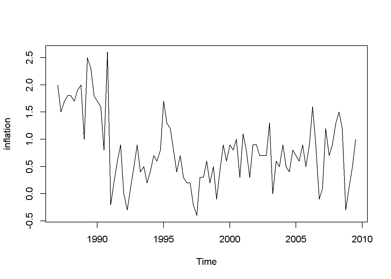
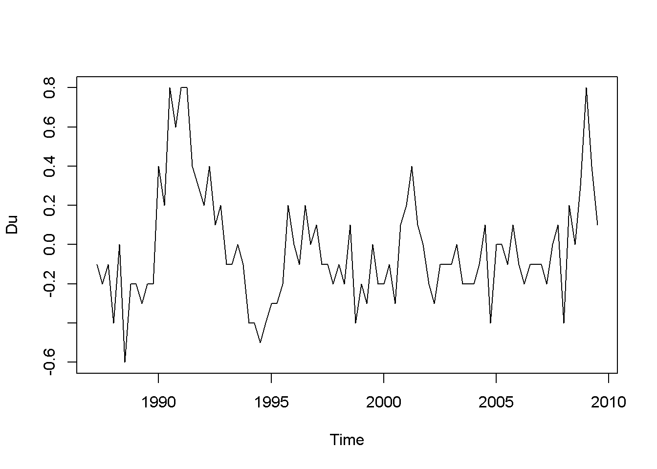
Figure 9.4: Data time plots in the ‘phillips’ dataset
The plots in Figure 9.4 definitely show patterns in the data for both inflation and unemployment rates. But we are interested to determine if the error term in Equation \ref{eq:philleq9} satisfies the non-autocorrelation assumption of the time series regression model.
phill.dyn <- dynlm(inf~diff(u),data=phill.ts)
ehat <- resid(phill.dyn)
kable(tidy(phill.dyn), caption="Summary of the `phillips` model")| term | estimate | std.error | statistic | p.value |
|---|---|---|---|---|
| (Intercept) | 0.777621 | 0.065825 | 11.81347 | 0.000000 |
| diff(u) | -0.527864 | 0.229405 | -2.30101 | 0.023754 |
Table 9.5 gives a \(p\)-value of \(0.0238\), which is significant at a $5% $ level. But is this \(p\)-value reliable? Let us investigate the autocorrelation structure of the errors in this model.
plot(ehat)
abline(h=0, lty=2)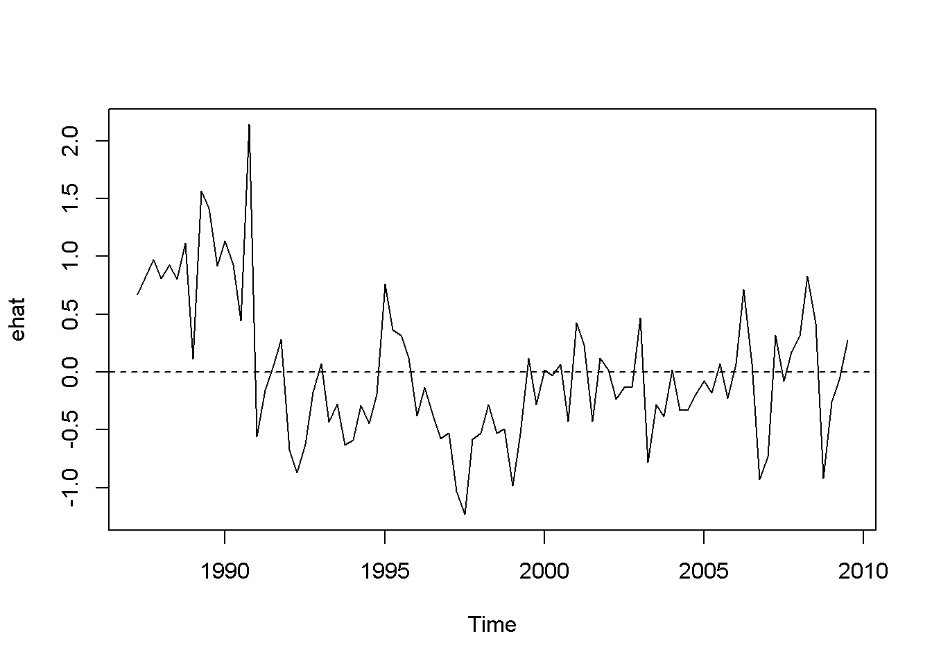
Figure 9.5: Residuals of the Phillips equation
corrgm <- acf(ehat)
plot(corrgm)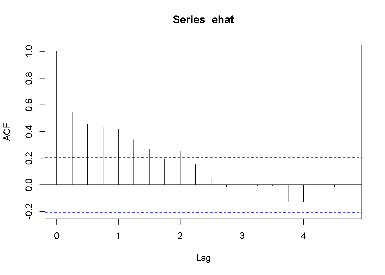
Figure 9.6: Correlogram of the residuals in the Phillips model
The time series plot in Figure 9.5 suggests that some patterns exists in the residuals, which is confirmed by the correlogram in Figure 9.6. The previous result suggesting that there is a significant relationship between inflation and change in unemployment rate may not be, afterall, too reliable.
While visualising the data and plotting the correlogram are powerful methods of spotting autocorrelation, in many applications we need a precise criterion, a test statistic to decide whether autocorrelation is a problem. One such a method is the Lagrange Multiplier test. Suppose we want to test for autocorrelation in the residuals the model given in Equation \ref{eq:bgeqinit9}, where we assume that the errors have the autocorrelation structure described in Equation \ref{eq:errstr9}.
\[\begin{equation} y_{t}=\beta_{1}+\beta_{2}x_{t}+e_{t} \label{eq:bgeqinit9} \end{equation}\] \[\begin{equation} e_{t}=\rho e_{t-1}+\nu _{t} \label{eq:errstr9} \end{equation}\]A test for autocorrelation would be based on the hypothesis in Equation \ref{eq:achyp9}.
\[\begin{equation} H_{0}:\rho =0,\;\;\;H_{A}:\rho \neq 0 \label{eq:achyp9} \end{equation}\]After little algebraic manipulation, the auxiliary regression that the LM test actually uses is the one in Equation \ref{eq:bgtesteq9}.
\[\begin{equation} \hat{e}_{t}=\gamma_{1}+\gamma_{2}x_{t}+\rho \hat{e}_{t-1}+\nu_{t} \label{eq:bgtesteq9} \end{equation}\]The test statistic is \(T\times R^2\), where \(R^2\) is the coefficient of determination resulted from estimating the auxiliary equation (Equation \ref{eq:bgtesteq9}). In \(R\), all these calculations can be done in one command, bgtest(), which is the Breusch-Godfrey test for autocorrelation function. This function can test for autocorrelation of higher orders, which requires including higher lags for \(\hat{e}\) in the auxiliary equation.
Let us do this test for the Phillips example. The next code sequence does the test first for only one lag and using an \(F\)-statistic; then, for lags up to 4, using a \(\chi^{2}\)-statistic. \(R\) does this test by either eliminating the first observations that are necessary to calculate the lags (fill=NA), or by setting them equal to zero (fill=0).
a <- bgtest(phill.dyn, order=1, type="F", fill=0)
b <- bgtest(phill.dyn, order=1, type="F", fill=NA)
c <- bgtest(phill.dyn, order=4, type="Chisq", fill=0)
d <- bgtest(phill.dyn, order=4, type="Chisq", fill=NA)
dfr <- data.frame(rbind(a[c(1,2,4)],
                  b[c(1,2,4)],
                  c[c(1,2,4)],
                  d[c(1,2,4)]
                  ))
dfr <- cbind(c("1, F, 0",
    "1, F, NA", "4, Chisq, 0", "4, Chisq, NA"), dfr)
names(dfr)<-c("Method", "Statistic", "Parameters", "p-Value")
kable(dfr, caption="Breusch-Godfrey test for the Phillips example")| Method | Statistic | Parameters | p-Value |
|---|---|---|---|
| 1, F, 0 | 38.4654 | 1, 87 | 1.82193e-08 |
| 1, F, NA | 38.6946 | 1, 86 | 1.73442e-08 |
| 4, Chisq, 0 | 36.6719 | 4 | 2.10457e-07 |
| 4, Chisq, NA | 33.5937 | 4 | 9.02736e-07 |
All the four tests summarized in Table 9.6 reject the null hypothesis of no autocorrelation. The above code sequence requires a bit of explanation. The first four lines do the BG test on the previously estimated Phillips model (phill.dyn), using various parametrs: order tells \(R\) how many lags we want; type gives the test statistic to be used, either \(F\) or \(\chi^{2}\); and, finally, fill tells \(R\) whether to delete the first observations or replace them with \(e=0\). The first column in Table 9.6 summarizes these options: number of lags, test statistic used, and how the missing observations are handeled.
The remaining of the code sequence is just to create a clear and convenient way of presenting the results of the four tests. As always, to inspect the content of an object like a type and run the command names(object).
How many lags should be considered when performing the autocorrelation test? One suggestion would be to limit the test to the number of lags that the correlogram shows to exceed the confidence band.
\(R\) can perform another autocorrelation test, Durbin-Watson, which is being used less and less today because of its limitations. However, it may be considered when the sample is small. The following command can be used to perform this test:
dwtest(phill.dyn)##
## Durbin-Watson test
##
## data: phill.dyn
## DW = 0.8873, p-value = 2.2e-09
## alternative hypothesis: true autocorrelation is greater than 09.5 Nonlinear Least Squares Estimation
The simple linear regression model in Equation \ref{eq:bgeqinit9} with AR(1) errors defined in Equation \ref{eq:errstr9} can be transformed into a model having uncorrelated errors, as Equation \ref{eq:nonlin9} shows.
\[\begin{equation} y_{t}=\beta_{1}(1-\rho)+\beta_{2}x_{t}+\rho y_{t-1}-\rho \beta_{2}x_{t-1}+\nu_{t} \label{eq:nonlin9} \end{equation}\]Equation \ref{eq:nonlin9} is nonlinear in the coefficients, and therefore it needs special methods of estimation. Applying the same transformations to the Phillips model given in Equation \ref{eq:philleq9}, we obtain its nonlinear version, Equation \ref{eq:phillnonlin9}.
\[\begin{equation} inf_{t}=\beta_{1}(1-\rho)+\beta_{2}Du_{t}+\rho inf_{t-1}-\rho \beta_{2}Du_{t-1}+\nu_{t} \label{eq:phillnonlin9} \end{equation}\]The next code line estimates the non-linear model in Equation \ref{eq:phillnonlin9} using the nls() function, which requires the data under a data frame form. The first few lines of code create a separate variables for inf and u and their lags, then brings all of them together in a data frame. The main arguments of the nls function are the following: formula, a nonlinear function of the regression parameters, data= a data frame, and `start=list(initial guess values of the parameters), and others.
library(dynlm)
phill.dyn <- dynlm(inf~diff(u), data=phill.ts)
# Non-linear AR(1) model with 'Cochrane-Orcutt method'nls'

phill.ts.tab <- cbind(phill.ts[,"inf"],
                      phill.ts[,"u"],
                      lag(phill.ts[,"inf"], -1),
                      diff(phill.ts[,"u"], lag=1),
                      lag(diff(phill.ts[,2],lag=1), -1)
                      )
phill.dfr <- data.frame(phill.ts.tab)
names(phill.dfr) <- c("inf", "u", "Linf", "Du", "LDu")
phill.nls <- nls(inf~b1*(1-rho)+b2*Du+rho*Linf-
                 rho*b2*LDu,
                 data=phill.dfr,
                 start=list(rho=0.5, b1=0.5, b2=-0.5))
s1 # This is `phill.dyn` with HAC errors:
##
## t test of coefficients:
##
## Estimate Std. Error t value Pr(>|t|)
## (Intercept) 0.77762 0.09485 8.198 1.82e-12 ***
## diff(u) -0.52786 0.30444 -1.734 0.0864 .
## ---
## Signif. codes: 0 '***' 0.001 '**' 0.01 '*' 0.05 '.' 0.1 ' ' 1phill.dyn # The simple linear model:##
## Time series regression with "ts" data:
## Start = 1987(2), End = 2009(3)
##
## Call:
## dynlm(formula = inf ~ diff(u), data = phill.ts)
##
## Coefficients:
## (Intercept) diff(u)
## 0.778 -0.528phill.nls # The 'nls' model:## Nonlinear regression model
## model: inf ~ b1 * (1 - rho) + b2 * Du + rho * Linf - rho * b2 * LDu
## data: phill.dfr
## rho b1 b2
## 0.557 0.761 -0.694
## residual sum-of-squares: 23.2
##
## Number of iterations to convergence: 3
## Achieved convergence tolerance: 8.06e-06coef(phill.nls)[["rho"]]## [1] 0.557398Comparing the nonlinear model with the two linear models (with, and without HAC standard errors) shows differences in both coefficients and standard errors. This is an indication that nonlinear estimation is a better choice than HAC standard errors. Please note that the NLS model provides an estimate of the autocorrelation coefficient, \(\rho=0.557\).
9.6 A More General Model
Equation \ref{eq:ardl9} gives an autoregresive distributed lag model, which is a generalization of the model presented in Equation \ref{eq:nonlin9}. The two models are equivalent under the restriction \(\delta_{1}=-\theta_{1}\delta_{0}\).
\[\begin{equation} y_{t}=\delta+\theta_{1}y_{t-1}+\delta_{0}x_{t}+\delta_{1}x_{t-1}+\nu_{t} \label{eq:ardl9} \end{equation}\]Equation \ref{eq:ardlphill9} is the Phillips version of the ARDL model given by Equation \ref{eq:ardl9}.
\[\begin{equation} inf_{t}=\delta+\theta_{1}inf_{t-1}+\delta_{0}Du_{t}+\delta_{1}Du_{t-1}+\nu_{t} \label{eq:ardlphill9} \end{equation}\]A Wald test can be used to decide if the two models, the nonlinear one and the more general one are equivalent.
s.nls <- summary(phill.nls)
phill.gen <- dynlm(inf~L(inf)+d(u)+L(d(u)),
                   data=phill.ts)
s.gen <- summary(phill.gen)
nlW <- nlWaldtest(phill.gen, texts="b[4]=-b[2]*b[3]")
The \(R\) function performing the Wald test is nlWaldtest in package nlWaldTest, which can test nonlinear restrictions. The result in our case is a \(\chi^2\) value of \(0.11227\), with \(p\)-value of \(0.737574\), which does not reject the null hypothesis that the restriction \(\delta_{1}=-\theta_{1}\delta_{0}\) cannot be rejected, making, in turn, Equations \ref{eq:phillnonlin9} and \ref{eq:ardlphill9} equivalent.
The code lines above use the L and d from package dynlm for constructing lags and differences in time series. Unlike the similar functions that we have previously used (lag and diff), these do not work outside the command dynlm. Please note that constructing lags with lag() requires specifying the negative sign of the lag, which is not necessary for the L() function..
phill1.gen <- dynlm(inf~lag(inf, -1)+diff(u)+lag(diff(u), -1), data=phill.ts)The results can be compared in Tables 9.8 and 9.9.
kable(tidy(phill.gen),
caption="Using dynlm with L and d operators")| term | estimate | std.error | statistic | p.value |
|---|---|---|---|---|
| (Intercept) | 0.333633 | 0.089903 | 3.71104 | 0.000368 |
| L(inf) | 0.559268 | 0.090796 | 6.15959 | 0.000000 |
| d(u) | -0.688185 | 0.249870 | -2.75417 | 0.007195 |
| L(d(u)) | 0.319953 | 0.257504 | 1.24252 | 0.217464 |
kable(tidy(phill1.gen),
caption="Using dynlm with lag and diff operators")| term | estimate | std.error | statistic | p.value |
|---|---|---|---|---|
| (Intercept) | 0.333633 | 0.089903 | 3.71104 | 0.000368 |
| lag(inf, -1) | 0.559268 | 0.090796 | 6.15959 | 0.000000 |
| diff(u) | -0.688185 | 0.249870 | -2.75417 | 0.007195 |
| lag(diff(u), -1) | 0.319953 | 0.257504 | 1.24252 | 0.217464 |
9.7 Autoregressive Models
An autoregressive model of order \(p\), \(AR(p)\) (Equation \ref{eq:autoregressivegen9}) is a model with \(p\) lags of the response acting as independent variables and no other regressors.
\[\begin{equation} y_{t}=\delta+\theta_{1}y_{t-1}+\theta_{2}y_{t-2}+...+\theta_{p}y_{t-p}+\nu_{t} \label{eq:autoregressivegen9} \end{equation}\]The next code sequence and Table 9.10 show an autoregressive model of order 2 using the series \(g\) in the data file \(okun\).
data(okun)
okun.ts <- ts(okun)
okun.ar2 <- dynlm(g~L(g)+L(g,2), data=okun.ts)
kable(tidy(okun.ar2), digits=4,
caption="Autoregressive model of order 2 using the dataset $okun$")| term | estimate | std.error | statistic | p.value |
|---|---|---|---|---|
| (Intercept) | 0.4657 | 0.1433 | 3.2510 | 0.0016 |
| L(g) | 0.3770 | 0.1000 | 3.7692 | 0.0003 |
| L(g, 2) | 0.2462 | 0.1029 | 2.3937 | 0.0187 |
How can we decide how many lags to include in an autoregressive model? One way is to look at the correlogram of the series and include the lags that show autocorrelation. The follwing code creates the correlogram in the AR(2) residuals of the US GDP series. The correlogram in Figure 9.7 shows that basically only the first two lags may be included.
res.ar2 <- resid(okun.ar2)
Acf(res.ar2, lag.max=12) # New: Acf() from package forecast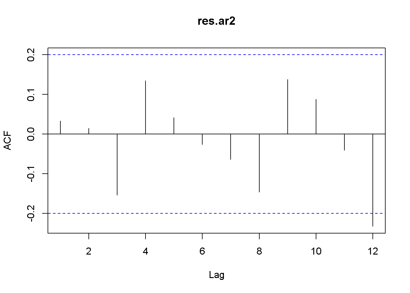
Figure 9.7: Residual correlogram for US GDP AR(2) model
Another way of choosing the specification of an autoregressive model is to compare models of several orders and choose the one that provides the lowest AIC or BIC value.
aics <- rep(0,5)
bics <- rep(0,5)
y <- okun.ts[,"g"]
for (i in 1:5){
  ari <- dynlm(y~L(y,1:i), start=i)
  aics[i] <- AIC(ari)
  bics[i] <- BIC(ari)
}
tbl <- data.frame(rbind(aics, bics))
names(tbl) <- c("1","2","3","4","5")
row.names(tbl) <- c("AIC","BIC")
kable(tbl, digits=1, align='c',
caption="Lag order selection for an AR model")| 1 | 2 | 3 | 4 | 5 | |
|---|---|---|---|---|---|
| AIC | 169.4 | 163.5 | 163.1 | 161.6 | 162.5 |
| BIC | 177.1 | 173.8 | 175.9 | 176.9 | 180.3 |
Table 9.11 displays the AIC and BIC (or SC) values for autoregressive models on the US GDP in dataset \(okun\) with number of lags from \(1\) to \(5\). (As mentioned before, the numbers do not coincide with those in PoE, but the ranking does.) The lowest AIC value indicates that the optimal model should include four lags, while the BIC values indicate the model with only two lags as the winner. Other criteria may be taken into account in such a situation, for instance the correlogram, which agrees with the BIC’s choice of model.
The previous code fragment needs some explanation. The first two lines initialize the vectors that are going to hold the AIC and BIC results. The problem of automatically changing the number of regressors is addressed by using the convenient function L(y, 1:i). AIC() and BIC() are basic \(R\) functions.
9.8 Forecasting
Let us consider first an autoregressive (AR) model, exemplified by the US GDP growth with two lags specified in Equation \ref{eq:gartwo9}.
\[\begin{equation} g_{t}=\delta+\theta_{1}g_{t-1}+\theta_{2}g_{t-2}+\nu_{t} \label{eq:gartwo9} \end{equation}\]Once the coefficients of this model are estimated, they can be used to predict (forecast) out-of-sample, future values of the response variable. Let us do this for periods \(T+1\), \(T+2\), and \(T+3\), where \(T\) is the last period in the sample. Equation \ref{eq:ar2forecast9} gives the forecast for period \(s\) into the future.
\[\begin{equation} g_{T+s}=\delta+\theta_{1}g_{T+s-1}+\theta_{2}g_{T+s-2}+\nu_{T+s} \label{eq:ar2forecast9} \end{equation}\]y <- okun.ts[,"g"]
g.ar2 <- dynlm(y~L(y, 1:2))
kable(tidy(g.ar2), caption="The AR(2) growth model")| term | estimate | std.error | statistic | p.value |
|---|---|---|---|---|
| (Intercept) | 0.465726 | 0.143258 | 3.25097 | 0.001602 |
| L(y, 1:2)1 | 0.377001 | 0.100021 | 3.76923 | 0.000287 |
| L(y, 1:2)2 | 0.246239 | 0.102869 | 2.39372 | 0.018686 |
Table 9.12 shows the results of the AR(2) model. \(R\) uses the function forecast() in package forecast to automatically calculate forecasts based on autoregressive or other time series models. One such model is ar(), which fits an autoregressive model to a univariate time series. The arguments of ar() include: x= the name of the time series, aic=TRUE, if we want automatic selection of the number of lags based on the AIC information criterion; otherwise, aic=FALSE; order.max= the maximum lag order in the autoregressive model.
ar2g <- ar(y, aic=FALSE, order.max=2, method="ols")
fcst <- data.frame(forecast(ar2g, 3))
kable(fcst, digits=3,
caption="Forcasts for the AR(2) growth model")| Point.Forecast | Lo.80 | Hi.80 | Lo.95 | Hi.95 | |
|---|---|---|---|---|---|
| 99 | 0.718 | 0.021 | 1.415 | -0.348 | 1.784 |
| 100 | 0.933 | 0.188 | 1.678 | -0.206 | 2.073 |
| 101 | 0.994 | 0.202 | 1.787 | -0.218 | 2.207 |
Table 9.13 shows the forecasted values for three future periods based on the AR(2) growth model.
plot(forecast(ar2g,3))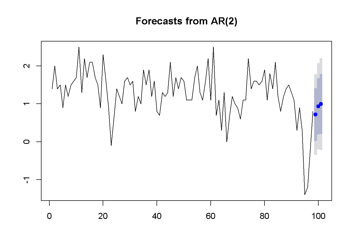
Figure 9.8: Forcasts and confidence intervals for three future periods
Figure 9.8 illustrates the forecasts produced by the AR(2) model of US GDP and their interval estimates.
Using more information under the form of additional regressors can improve the accuracy of forecasting. We have already studied ARDL models; let us use such a model to forecast the rate of unemployment based on past unemployment and GDP growth data. The dataset is still \(okun\), and the model is an ARDL(1,1) as the one in Equation \ref{eq:ardlfcst9}.
\[\begin{equation} Du_{t}=\delta+\theta_{1}Du_{t-1}+\delta_{0}g_{t}+\delta_{1}g_{t-1}+\nu_{t} \label{eq:ardlfcst9} \end{equation}\]Since we are interested in forecasting levels of unemployment, not differences, we want to transform the ARDL(1,1) model in Equation \ref{eq:ardlfcst9} into the ARDL(2,1) one in Equation \ref{eq:ardllevelfcst9}.
\[\begin{equation} u_{T+1}=\delta+\theta_{1}^*u_{T}+\theta_{2}^*u_{T-1} +\delta_{0} g_{T+1}+\delta_{1}g_{T}+\nu_{T+1} \label{eq:ardllevelfcst9} \end{equation}\]Another forecasting model is the exponential smoothing one, which, like the AR model, uses only the variable to be forecasted. In addition, the exponential smoothing model requires a weighting parameter, \(\alpha\), and an initial level of the forecasted variable, \(\hat y\). Next period’s forecast is a weighted average of this period’s level and this period’s forecast, as indicated in Equation \ref{eq:expsmoothing9}.
\[\begin{equation} \hat{y}_{T+1}=\alpha y_{T}+(1-\alpha)\hat{y}_{T} \label{eq:expsmoothing9} \end{equation}\]There are sevaral ways to compute an exponential smoothing forecast in \(R\). I only use two here, for comparison. The first is the function ets() in the forecast package.
y <- okun.ts[,"g"]
okun.ets <- ets(y)
okunf.ets <- forecast(okun.ets,1) #one-period forecast
plot(okunf.ets)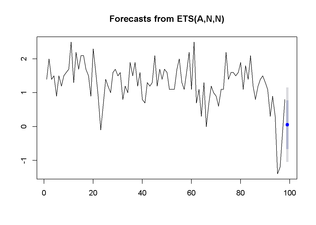
Figure 9.9: Exponential smoothing forecast using ‘ets’
The results include the computed value of the weight, \(\alpha=0.381\), the point estimate of the growth rate \(g_{T+1}=0.054\), and the 95 percent interval estimate \((-1.051, 1.158)\). Figure 9.9 illustrates these results.
The second method uses the function HoltWinters and is shown in the following code fragment.
okun.HW <- HoltWinters(y, beta=FALSE, gamma=FALSE)
plot(okun.HW)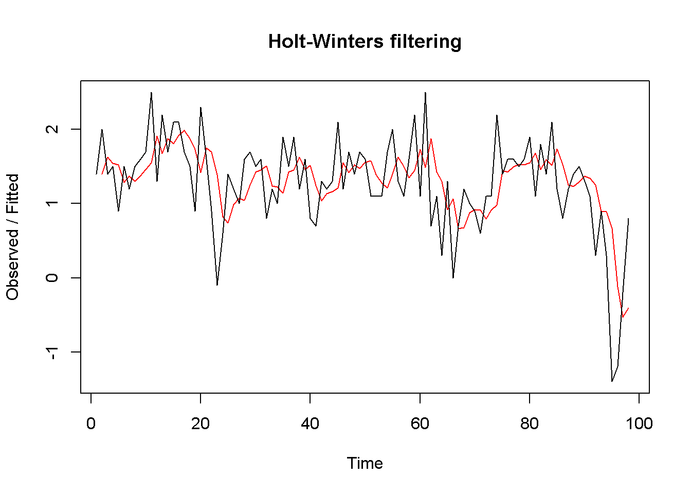
Figure 9.10: Exponential smoothing forecast using ‘HoltWinters’
okunf.HW <- forecast(okun.HW,1)Similar to the ets function, HoltWinters automatically determines the optimal weight \(\alpha\) of the exponential smoothing model. In our case, the value is \(\alpha = 0.381\). The point estimate is \(g_{T+1}=0.054\), and the 95 percent interval estimate is \((-1.06,1.168)\). Figure 9.10 compares the forecasted with the actual series.
9.9 Multiplier Analysis
In an \(ARDL(p,q)\) model, if one variable changes at some period it affects the response over several subsequent periods. Multiplier analysis quantifies these time effects. Let me remind you the form of the \(ARDL(p,q)\) model in Equation \ref{eq:ardlpqgen9}.
\[\begin{equation} y_{t}=\delta +\theta_{1}y_{t-1}+...+\theta_{p} y_{t-p}+\delta_{0}x_{t}+ \delta_{1}x_{t-1}+...+\delta_{q}x_{t-q}+\nu_{t} \label{eq:ardlpqgen9} \end{equation}\]The model in Equation \ref{eq:ardlpqgen9} can be transformed by iterative substitution in an infinite distributed lag model, which includes only explanatory variables with no lags of the response. The transformed model is shown in Equation \ref{eq:infdlmodel9}.
\[\begin{equation} y_{t}=\alpha+\beta_{0}x_{t}+\beta_{1}x_{t-1}+\beta_{2}x_{t-2}+\beta_{3}x_{t-3}+...+e_{t} \label{eq:infdlmodel9} \end{equation}\]Coefficient \(\beta_{s}\) in Equation \ref{eq:infdlmodel9} is called the s-period delay multiplier; the sum of the \(\beta\)s from today to period \(s\) in the past is called interim multiplier, and the sum of all periods to infinity is called total multiplier.
References
Zeileis, Achim. 2016. Dynlm: Dynamic Linear Regression. https://CRAN.R-project.org/package=dynlm.
Spada, Stefano, Matteo Quartagno, and Marco Tamburini. 2012. Orcutt: Estimate Procedure in Case of First Order Autocorrelation. https://CRAN.R-project.org/package=orcutt.
Komashko, Oleh. 2016. NlWaldTest: Wald Test of Nonlinear Restrictions and Nonlinear Ci. https://CRAN.R-project.org/package=nlWaldTest.
Reinhart, Abiel. 2015. Pdfetch: Fetch Economic and Financial Time Series Data from Public Sources. https://CRAN.R-project.org/package=pdfetch.
Hyndman, Rob. 2016. Forecast: Forecasting Functions for Time Series and Linear Models. https://CRAN.R-project.org/package=forecast.