Chapter 1 Jan 3–9: Handling Data in R, Linear Relationships Review

This chapter is now updated and ready for HE-902 students to use in spring 2022.

This chapter contains the only content that you need to look at for the first week of the course, which is January 3–9 2022. You can ignore all subsequent chapters in this textbook, for now.

Please read this entire chapter and then complete the assignment at the end. As you read, I recommend that you copy and paste all of the code into RStudio on your own computer, both to practice and to make it easier to do the assignment.

Since this is an advanced, PhD-level course, the first few weeks will include a review of basic statistical and math concepts at a fast pace.

I recommend that you quickly skim through the assignment at the end of the chapter before going through this chapter’s content, so that you know in advance the tasks that you will be expected to do.

This week, our goals are to…

Become familiar with this textbook and the structure of the course.
Import, explore, and manipulate data in R and RStudio.
Review basic linear relationships and linear equations, including the meaning of slope and intercept.

Please continue to the next section to begin your work in this course!

1.1 Course basics

Since this is the first week of the course, we will go over a few administrative and workflow items now. Please start by watching the following embedded video:

The video above can also be viewed externally at https://youtu.be/1pjbnUzItXk.

Please also watch the following video which demonstrates how you can use this textbook and RStudio together:

The video above can also be viewed externally at https://youtu.be/dt-YzmApiyE.

Below is some information about how to use this textbook and how the course will work on a weekly basis.

If you did not attend an orientation/welcome session already, please inform all course instructors so that we can schedule an orientation session for you.
Like most other courses in the PhD program in Health Professions Education at MGHIHP, this is an online asynchronous course. This means that there are no regularly scheduled class meetings. Instead, you and your fellow students will consume each week’s learning materials and complete all assignments according to your own preferred schedule within each week. We will also hold optional (not required) “office hour” meetings on Zoom each week which you can attend if you have questions and/or would like to work together with your classmates.
The introductory chapter of this textbook contains information about the course. Please read it if you have not done so already. The course calendar, final project, and oral exams sections might be particularly useful. You can also review everything we did during the R and RStudio orientation session.
Throughout this textbook, you will find many links that you can click on. These are marked in blue underlined text like this. Any time you see blue text like that, keep in mind that you can click on it! You can practice by clicking here.
Each week of the course, a chapter of this textbook will be assigned for you to use. This week—the week of January 3–9 2022—the assigned chapter is Chapter 1, the one you are reading right now. You can look up which chapter is assigned for each week in the course calendar in the introductory chapter. This week, you should read through all of the text in this chapter, watch any videos, and then complete the assignment at the end of the chapter. Everything you need to do this week is exclusively in this chapter. And you will do the same for chapters assigned in future weeks.
The due date of each assignment is usually Sunday night at the end of each week. Assignment due dates are given in the course calendar in the introductory chapter. Assignments should be submitted in D2L. Any other submission instructions will be included in each individual assignment.
For the majority of this course, as you go through each chapter, you will encounter R code. As you read, I highly recommend that you copy and paste all provided R code into an R file on your own computer and run it on your own computer. This will not only help you practice you data analysis skills but also make it easier and faster for you to do each assignment. Remember that you should paste/write all of your code into an R script file and then save your work in that file as you go. DO NOT type your code directly into the console, because then it will not be saved.
Sometimes in this online textbook, the code provided is for illustrative purposes only and may not run for you when you copy and paste it into RStudio on your own computer. Nevertheless, I recommend that you still paste all code into RStudio into your own computer as you read, so that you have it available for future use, including when you do the assignment at the end of the chapter.
In RStudio, note that you can customize the layout. For example, you can click on View -> Panes -> Console on Right to move RStudio’s console to the right side of the screen. I personally prefer the console to be on the right side. In some of the instructional videos you watch in this course, the layout of RStudio might be a little bit different from how you have it on your own computer.
If you find that the work for a given week is taking you too long, I recommend that you stop and send an e-mail to all course instructors. For example, if you get stuck on the first few lines of code and realize that you have spent a long time trying to debug them but you still can’t get them to run properly, I recommend that you stop at that point (or even sooner) and contact us. We can meet on Zoom and work through a section of the code and/or content with you so that you finish at a pace that is reasonable for your schedule. Please overcommunicate with us rather than undercommunicate. Do not hesitate to contact us!

Now you are ready to start the course, by reading the rest of this chapter and then doing the assignment at the end!

1.2 Selected R functionality and operations

During the orientation procedure, we downloaded R and RStudio, ran some basic operations, loaded the built-in dataset mtcars, and created a few descriptive tables and visualizations. In this section, we will learn about a few additional basic functionalities in R that we will be using on a regular basis.

You might be wondering about what R and RStudio are exactly. Here are some key distinctions:

R is the programming language that we will use to do all of our work. All of the code that you will write and run will be in the R programming language. You can think of R just like a language like English, which we write using numbers, letters, and symbols. When someone asks you which software you used to do your analysis, you should say, “I used R.”
RStudio is a software that we use to help us use the programming language R. RStudio makes it easier to write R code and also provides us with a number of additional tools to do our work. While R is a language like English, RStudio is a tool—analogous to Microsoft Word—that we use to write that language. When someone asks you which software you used to do your analysis, you should NOT say: “I used RStudio.” You should say: “I used R.”¹²

When you are doing work for this course, ALWAYS open the program called “RStudio” on your computer. DO NOT open the program called “R” or anything else.

1.2.1 Functions

Many of the actions that you will do in R will use functions. A function will have its own unique name, such as table or lm or SomeOtherName. When you use a function, you will type the name of the function and then parentheses. Within those parentheses, you will often—but not always—write some more instructions. These instructions within the parentheses are called arguments. Arguments should be separated by commas. Two examples are below.

Example with table(...) function:

table(mtcars$vs, mtcars$am)

Above, we told the computer to run the table function and it contained two arguments: mtcars$vs and mtcars$am.

Example with a hypothetical function called SomeOtherName, for illustrative purposes only:

SomeOtherName(data = df, title = "cats have one life each",'AuntArtIca', mustard, worms)

The code above is completely fake and made up. Nevertheless, it follows the logic of R code and functions in R. Above, we are telling the computer to run the hypothetical function SomeOtherName and we are giving five arguments to the function, within parentheses and separated by commas. These five arguments are all very different from each other, which is common in R commands that you might write.

Note that in situations where quotation marks are used, both single (') and double (") quotation marks can be used interchangeably. In the function above, the words cats have one life each are surrounded by double quotation marks but they could be surrounded by single quotation marks (like AuntArtIca is) and that would also be fine.

You will encounter a huge variety of functions and arguments within those functions as you continue to use R.

1.2.2 Installing and loading packages

When you download R to your computer, it comes along with many possible commands and analysis options that you can use. Quite often, you will find the need to run additional commands that did not come with R when you downloaded it. To add functionality to R on your computer, we have to install what are called packages.

To install a package to your computer, you will run a command like this:

if (!require(packagename)) install.packages('packagename')

In the code above, you would replace the word packagename with the actual name of the package you want to install. The code above checks whether a package is already on your computer or not. If it is not, the package will get installed to your computer. If it is already on your computer, nothing will happen.

If you want to force the computer to install a package no matter what, you can run this code:

install.packages('packagename')

Once a package is on your computer, you can load it using the library(...) function:

library(packagename)

When you are using the code above on your own, you would replace the word packagename with the name of the package you want to load.

My favorite way to use a package is with the following two lines of code:

if (!require(packagename)) install.packages('packagename')
library(packagename)

The code above should take care of everything. Just replace packagename—in all three places where it appears above—with the name of the package you want to load.

What is the difference between installing and loading a package?

Installing: Installing a package—if (!require(packagename)) install.packages('packagename')— is like going to a hardware store, buying a new toolbox full of tools, bringing it home and putting it in the closet. You can also think of it as analogous to downloading an app from the app store to your smartphone. A new package only needs to be installed once.
Loading: Loading a package—library(packagename)---is like going to your closet, getting a toolbox, and opening the toolbox so that you are ready to use the tools inside. You can also think of this as analogous to going to the home screen and opening an app that has already been downloaded to your smartphone, but had not been open recently. *Every time* you want to use a package, you have to load it again using thelibrary(…)` function.

1.3 Loading and exploring data in R

In this section of the chapter, we will learn how to set R’s working directory, load data from an Excel file into R, make descriptive tables, subset our data, transform variables (columns in our data), recode variables, and remove duplicate observations (rows in our data). You will also practice skills such as installing and loading any required R packages, writing code into an R script file, and saving your work.

As you go through this section of this chapter, I recommend that you follow along by copying and pasting all of the provided code below into your own R file on your own computer.

1.3.1 Set the working directory in R and RStudio

As you practiced during our orientation session, R can interact with files on your computer. You practiced saving an R script file on your computer. To save the file, you had to tell your computer a folder in which you wanted to save the file. Note that directory is another name for folder (on your computer).

When you are loading files from and saving files to your computer, you need to tell R where on your computer to look for those files. The place where R will look is called the working directory. Any time you start using R, you should set the working directory. This will be done using a line of code which you can keep towards the top of the code file you are using.

Here is the function that you can use to set the working directory on your computer:

setwd("C:/path/on/your/computer/to/a/folder")

Above, you will replace C:/path/on/your/computer/to/a/folder with an actual file path on your computer. There are a number of ways to do this in RStudio.

To figure out what the current working directory on your computer is—both before and after you run the setwd() command—you can run the following function:

getwd()

Please watch the video below which shows multiple methods of how to set your working directory in R and RStudio.

The video above can also be viewed externally at https://youtu.be/_YK6Gwvr1Fw or https://tinyurl.com/RStudioSetWD.

Remember that you only need to know one way to set your working directory in R and RStudio. You can choose whichever way is best for you. You do not need to use all of the methods demonstrated in the video, just one.

In the video, the command used to set the working directory is:

setwd("C:/My Data Folder/Project1")

Above, I had a folder on my computer that was called Project1 which was located in another folder called My Data Folder which was on my C: drive. Perhaps you have created a folder for all the work you do in this course, in which case you can set that folder as your working directory using the setwd() command like I did above, but with a different file path within the quotation marks.

It is also possible to see a list of all of the files within your working directory by running the following code:

list.files()

The result of the code above is not shown. If you run the list.files() function (with no arguments included) on your own computer, you should get a list of files in your working directory (which is where R will look for files if you ask it to).

Remember that a folder is different from a file. A folder is a container on your computer that holds files. Work you do in Microsoft Word, Excel, and R are saved in individual files. Those files are then saved in folders on your computer. A directory is the same thing as a folder. setwd stands for “set working directory,” which means “set the folder where R should look for stuff.” When you set the working directory, you have to put a folder—not a file—inside the quotation marks in the setwd() function.

1.3.2 Load Excel data into R

Loading data into R from an Excel file is a very useful skill that you are likely to need both in our course and in your own quantitative analysis work in the future. As with most processes in R, there are multiple ways to do this. Two methods are shown below, but you only need to know one. In most cases, either of these methods will accomplish what you need to do. I have included a video that shows how to do this for one of the methods.

Of course, before you load data from Excel into R, you first need to have an Excel data file to load. Please follow the procedure below:

Click here to download an Excel file.¹³
Save the downloaded file in your working directory, the same working directory you designated in the earlier section. The file is a ZIP file called sampledatafoodsales.zip.
Open the file sampledatafoodsales.zip and you should find an Excel file within it called sampledatafoodsales.xlsx.
Copy sampledatafoodsales.xlsx into your working directory.
Open the file sampledatafoodsales.xlsx in Excel (not R or RStudio) to see what it is like.
Notice that the data file (in Excel) contains three sheets. The data we want is in the second sheet, called FoodSales.

Now you are ready to load the Excel data in sampledatafoodsales.xlsx into R using one of the two methods below. If one of the methods doesn’t work, try the other! It is fine if only one method works for you.

1.3.2.1 Method 1 – readxl package

This method uses the readxl package to load data from an Excel file into R. This is my favorite way to load Excel data into R.

The video below goes through the procedure, in case you wish to watch rather than read about it:

The video above can also be viewed externally at https://youtu.be/AxDcbmxQnxE or https://tinyurl.com/LoadExcelRStudio.

Below is a written explanation of the procedure to load Excel data into R using the readxl package.

You can begin the procedure by loading the readxl package with the following code:

if (!require(readxl)) install.packages('readxl')
library(readxl)

Remember, any time I give you some code, you should copy and paste it into your own code file in RStudio on your own computer! Be sure to copy the lines of code above—and all subsequent lines of code—into your own code file.

Let’s review the two lines of code above:

if (!require(readxl)) install.packages('readxl') – This line checks if the package readxl is already installed on your computer. If it is not, then it installs the package for you. Keep in mind that installing a new package can often take many minutes.
library(readxl) – This line loads the readxl package into your current session of R. By the time we get to this line, the readxl package should be installed already, because either it was already on your computer or it was installed by the previous line of code.

Now that the package is installed and loaded, you can load the Excel file from the working directory, using the code below:

dat<- read_excel("sampledatafoodsales.xlsx", sheet = "FoodSales")

Above, we created a new dataset in R (technically called a data frame) which is called dat. We could have called it anything else we wanted, different than dat. Our new dataset dat contains the data in the sheet called FoodSales in the Excel file called sampledatafoodsales.xlsx.

Here are some more detailed notes about what we did:

You can change dat to whatever you want your dataset to be called in R. This name should show up in RStudio’s Environment tab once you run the command.
The read_excel() function has two arguments in the code above. Let’s go through them:
- file="sampledatafoodsales.xlsx" – This tells the computer which Excel file you want it to look at, within the working directory.
- sheet = "FoodSales" – This tells the computer to look at the sheet called FoodSales within the Excel file.

1.3.2.2 Method 2 – xlsx package

This method uses the xlsx package, which you can load by running the following code:

if (!require(xlsx)) install.packages('xlsx')
library(xlsx)

Let’s review the two lines of code above:

if (!require(xlsx)) install.packages('xlsx') – This line checks if the package xlsx is already installed on your computer. If it is not, then it installs the package for you. Keep in mind that installing a new package can often take many minutes.
library(xlsx) – This line loads the xlsx package into your current session of R. By the time we get to this line, the xlsx package should be installed already, because either it was already on your computer or it was installed by the previous line of code.

Now that the package is installed and loaded, you can load the Excel file from the working directory, using the code below:

d <- read.xlsx(file="sampledatafoodsales.xlsx", sheetIndex = 2, header=TRUE)

Above, we created a new dataset in R (technically called a data frame) which is called d. We could have called it anything else we wanted, different than d. Our new dataset d contains the data in the second sheet of the Excel file called sampledatafoodsales.xlsx.

Here are some more detailed notes about what we did:

You can change d to whatever you want your dataset to be called in R. This name should show up in RStudio’s Environment tab once you run the command.
The read.xlsx() function has three arguments in the code above. Let’s go through them:
- file="sampledatafoodsales.xlsx" – This tells the computer which Excel file you want it to look at, within the working directory.
- sheetIndex = 2 – This tells the computer to look at the second sheet within the Excel file. If you want it to look at sheet #3, change the 2 to 3 in this code.
- header=TRUE – This tells the computer that the very first row of your Excel file contains variable names, and not raw data.

1.3.2.3 Double-check your data

Once your data is loaded into R from the Excel file, you should double-check to make sure that it was loaded correctly. Let’s say that you named your data file dat, as in one of the examples above. You should be able to see a new Data item within the Environment tab in RStudio. You can double-click on dat within the Environment tab and a data viewer should pop up, showing you your Excel data within RStudio itself.

Another way to view the data is to run the following command:

View(dat)

Running the command above should also open up a data viewer in RStudio for you to view your data. If you named your data something other than dat, then replace dat with your data’s name in the command above. For example: View(someothername).

Compare your data in the RStudio viewer with the data in Excel. It should be identical. Always be sure to double-check everything before you proceed!

If you want to just look at the first few rows of your dataset, you can use the head(...) function:

head(dat, n=10)

## # A tibble: 10 x 8
##    OrderDate           Region City       Category Product     Quantity UnitPrice
##    <dttm>              <chr>  <chr>      <chr>    <chr>          <dbl>     <dbl>
##  1 2020-01-01 00:00:00 East   Boston     Bars     Carrot            33      1.77
##  2 2020-01-04 00:00:00 East   Boston     Crackers Whole Wheat       87      3.49
##  3 2020-01-07 00:00:00 West   Los Angel~ Cookies  Chocolate ~       58      1.87
##  4 2020-01-10 00:00:00 East   New York   Cookies  Chocolate ~       82      1.87
##  5 2020-01-13 00:00:00 East   Boston     Cookies  Arrowroot         38      2.18
##  6 2020-01-16 00:00:00 East   Boston     Bars     Carrot            54      1.77
##  7 2020-01-19 00:00:00 East   Boston     Crackers Whole Wheat      149      3.49
##  8 2020-01-22 00:00:00 West   Los Angel~ Bars     Carrot            51      1.77
##  9 2020-01-25 00:00:00 East   New York   Bars     Carrot           100      1.77
## 10 2020-01-28 00:00:00 East   New York   Snacks   Potato Chi~       28      1.35
## # ... with 1 more variable: TotalPrice <dbl>

In the code above, we put dat and n=10 as two separate arguments¹⁴ into the head(...) function. This tells the computer to take the dataset dat and display the first 10 rows of it for us. If we had changed the number 10 to a different number, like 15, then it would show us the first 15 rows of the data.

If you want your entire dataset to be outputted by R, you can simply type the name of the dataset into a line of code and run it, like this:

dat

The result of the code above is not shown, because it would be too long and not useful for us. All 244 rows of the dataset would have been displayed. You can try this on your own computer as you follow along.

Now that you have loaded data into R, the next sections will show you how to explore and manipulate this data.

1.3.3 Explore our data

Below, you will learn how to explore selected aspects of any data that you have loaded into R, such as the looking up the number of rows and columns and the names of all variables (columns). In the examples below, the name of the data that we are using in R is dat. But you can replace dat with any other name such as d, mydata, mtcars, AnyNameYouDecide.

Since we have already loaded a dataset called dat above, we will continue to use dat as our example dataset in this chapter. When you do analysis of your own, the name of your dataset might be something other than dat, so you can replace the word dat with the name of your own dataset when you use the R commands shown below. Your data will also contain variables (columns) with different names than the variables in the examples below. You can write your own dataset’s variable’s names in place of the ones in the examples.

1.3.3.1 Size of dataset

Let’s start by looking up the number of rows in the data:

nrow(dat)

## [1] 244

Above, using the nrow() function, we asked the computer to tell us how many rows are in the dataset dat. It told us that there are 244 rows. A row of data is also called an observation.

Next, let’s look up the number of columns in the data:

ncol(dat)

## [1] 8

Above, using the ncol() function, we asked the computer to tell us how many columns are in the dataset dat. It told us that there are 8 columns. A column of data is also called a variable.

There is also a way to look up the rows and columns simultaneously:

dim(dat)

## [1] 244   8

Above, the computer told us that dat contained 244 rows (observations) and 8 columns (variables).

1.3.3.2 Variable names and characteristics

As mentioned above, each column represents a variable. A variable is a characteristic that we have recorded about each observation. Each variable has a name, which is listed in the very first row of the spreadsheet in which the data is kept.

You can quickly view the names of all of the variables in your data using the following command:

names(dat)

## [1] "OrderDate"  "Region"     "City"       "Category"   "Product"   
## [6] "Quantity"   "UnitPrice"  "TotalPrice"

As you can see above, when we ran the names() function on our dataset dat, the computer printed out all of the names of the 8 variables.

We can also use the str(...) function to learn more about our dataset dat:

str(dat)

## tibble[,8] [244 x 8] (S3: tbl_df/tbl/data.frame)
##  $ OrderDate : POSIXct[1:244], format: "2020-01-01" "2020-01-04" ...
##  $ Region    : chr [1:244] "East" "East" "West" "East" ...
##  $ City      : chr [1:244] "Boston" "Boston" "Los Angeles" "New York" ...
##  $ Category  : chr [1:244] "Bars" "Crackers" "Cookies" "Cookies" ...
##  $ Product   : chr [1:244] "Carrot" "Whole Wheat" "Chocolate Chip" "Chocolate Chip" ...
##  $ Quantity  : num [1:244] 33 87 58 82 38 54 149 51 100 28 ...
##  $ UnitPrice : num [1:244] 1.77 3.49 1.87 1.87 2.18 1.77 3.49 1.77 1.77 1.35 ...
##  $ TotalPrice: num [1:244] 58.4 303.6 108.5 153.3 82.8 ...

str stands for structure. The str(...) function can be used to examine a variety of stored objects in R, not only datasets like dat. In the output above, we see a list of all variables as well as some details about each variable. We see that variables like Region and City are variables of type chr, which stands for character. Character variables contain words and letters. Qualitative categorical variables like Region and City are often coded as chr or factor variables. Variables like Quantity and UnitPrice are numeric variables, which is why they are labled as num.

It is also possible to look up some specific details of a single variable. We can determine a variable’s type by using the class(...) function:

class(dat$Region)

## [1] "character"

Above, the computer tells us that the variable Region within the dataset dat is a character variable. This tells us that Region is not a numeric variable and is instead a qualitative categorical variable.

Looking up the number of rows, number of columns, names of columns (variables), and variable types in your data are important processes to keep in mind and use on a regular basis as you do your data analysis.

1.3.4 One-way tables

Another very important tool is a table. A table will tell you how your observations fall into categories of a particular variable. It is easiest to start with an example.

You can run the following code to make a one-way table:

table(dat$City)

## 
##      Boston Los Angeles    New York   San Diego 
##          88          55          62          39

Here is what we did with the code above:

We used the table() function to tell the computer to make a table.
We had to tell the computer what to make a table of, by putting something into the parentheses within the table() function. We told the computer that we wanted it to make a table based on the City variable within the dataset dat.

The computer then broke down the 244 observations in the dataset dat into the four possible values of City that an observation can have. For example, we know that 62 observations have New York as their City.

If we wanted to, we could change City in the code above to a different variable, like this:

table(dat$Region)

## 
## East West 
##  150   94

Above, the computer now broke down all 244 observations according to the variable Region.

What if we make a table of the variable Quantity? Let’s try it.

table(dat$Quantity)

## 
##  20  21  22  23  24  25  26  27  28  29  30  31  32  33  34  35  36  37  38  39 
##   7   5   2   4   4   4   3   6   6   5  10   6   4   6   6   1   4   1   8   3 
##  40  41  42  43  44  45  46  47  48  49  50  51  52  53  54  55  56  57  58  60 
##   7   5   4   4   4   1   1   3   2   3   1   4   2   1   1   2   3   2   6   1 
##  61  62  63  64  65  66  67  68  70  71  72  73  74  75  76  77  79  80  81  82 
##   2   1   2   2   4   1   1   4   1   1   1   1   1   3   1   3   1   2   1   2 
##  83  84  85  86  87  90  91  92  93  96  97 100 102 103 105 107 109 110 114 118 
##   2   1   1   2   2   3   1   1   1   1   2   2   1   3   1   1   1   2   1   1 
## 120 123 124 129 133 134 136 137 138 139 141 143 146 149 175 193 211 224 232 237 
##   1   2   1   1   1   1   2   2   1   2   1   1   1   1   1   1   1   1   1   1 
## 245 288 306 
##   1   1   1

Above, we received an enormous table from the computer which isn’t that helpful to us. City and Region are categorical variables that allow us to easily group our observations. Quantity is a continuous numeric variable and most observations have a unique value for Quantity, so making a table isn’t as useful.

What if you want to slice your data according to more than just one variable? That’s where two-way tables come in. Keep reading!

1.3.5 Two-way tables

A two-way table is very similar to a one-way table, except it allows you to use two variables to divide up your observations. Let’s see an example.

You can run the following code to make a two-way table:

table(dat$City, dat$Region)

##              
##               East West
##   Boston        88    0
##   Los Angeles    0   55
##   New York      62    0
##   San Diego      0   39

Here is what we did with the code above:

We used the table() function to tell the computer to make a table.
We had to tell the computer what to make a table of, by putting something into the parentheses within the table() function. We told the computer that we wanted it to make a table with a) the City variable within the dataset dat in the rows and b) the Region variable within the dataset dat in the columns.

The computer then broke down the 244 observations in the dataset dat into the four possible values of City that an observation can have and the two possible values of Region that an observation can have. For example, we know that 55 observations have Los Angeles as their City and West as their Region. 0 cities have Los Angeles as their City and East as their Region.

You may have noticed that the two-way table above does not label which variable is shown in the rows and columns. Sometimes, this can make it confusing to figure out which variable is in which place. If we use the with(...) function and put the table function within it, we can add variable labels.

Here we put the table(...) function within the with(...) function to make a two-way table with labels:

with(dat, table(City, Region))

##              Region
## City          East West
##   Boston        88    0
##   Los Angeles    0   55
##   New York      62    0
##   San Diego      0   39

While the table(...) function is a convenient way to make tables that is built into R, there are also other ways to make tables. One way is the cro(...) function from the expss package.

This code recreates the two-way table above using cro(...):

if (!require(expss)) install.packages('expss')
library(expss)

cro(dat$City, dat$Region)

	dat$Region
	East	West
dat$City
Boston	88
Los Angeles		55
New York	62
San Diego		39
#Total cases	150	94

1.3.6 Percentage tables

It is also possible to make one-way and two-way tables that show percentages instead of counts. Please see below for examples and code.

Let’s start with a one-way table of the variable Category from the dataset dat, using the code below:

table(dat$Category)

## 
##     Bars  Cookies Crackers   Snacks 
##       94       95       26       29

To convert the table above to a table with proportions, we will take the code above—table(dat$Category)—and put it all inside of the prop.table(...) function, as shown here:

prop.table(table(dat$Category))

## 
##      Bars   Cookies  Crackers    Snacks 
## 0.3852459 0.3893443 0.1065574 0.1188525

Above, the one-way table now shows proportions of observations in each category, as fractions of 1.

Finally, we can multiply the entire table by 100, such that it shows percentages:

prop.table(table(dat$Category))*100

## 
##     Bars  Cookies Crackers   Snacks 
## 38.52459 38.93443 10.65574 11.88525

Above, we see that for the variable Category, 38.9% of all observations have the level Cookies. This means that 38.9% of orders were for cookies. Optionally (not required), see this sentence’s footnote regarding reducing the number of displayed decimal places.¹⁵

We will now turn to two-way tables, starting with this two-way table of City and Category:

table(dat$City, dat$Category)

##              
##               Bars Cookies Crackers Snacks
##   Boston        29      32       17     10
##   Los Angeles   24      22        2      7
##   New York      26      22        5      9
##   San Diego     15      19        2      3

Again, we will use the prop.table(...) function to convert the table above into a proportion table:

prop.table(table(dat$City, dat$Category))

##              
##                      Bars     Cookies    Crackers      Snacks
##   Boston      0.118852459 0.131147541 0.069672131 0.040983607
##   Los Angeles 0.098360656 0.090163934 0.008196721 0.028688525
##   New York    0.106557377 0.090163934 0.020491803 0.036885246
##   San Diego   0.061475410 0.077868852 0.008196721 0.012295082

And like before we can multiply this entire table by 100 to get percentages:

prop.table(table(dat$City, dat$Category))*100

##              
##                     Bars    Cookies   Crackers     Snacks
##   Boston      11.8852459 13.1147541  6.9672131  4.0983607
##   Los Angeles  9.8360656  9.0163934  0.8196721  2.8688525
##   New York    10.6557377  9.0163934  2.0491803  3.6885246
##   San Diego    6.1475410  7.7868852  0.8196721  1.2295082

The table above tells us that 13.1% of all observations have a City value of Boston and a Category value of Cookies. More plainly: 13.1% of all orders are cookies sent to Boston. Note that the table above has 4 rows and 4 columns, meaning it has 16 cells in total. The total sum of the numbers in all 16 cells adds up to 100%.

Alternatively, you can calculate the percentages by row or column. Let’s do row percentages first, using this code:

prop.table(table(dat$City, dat$Category), margin = 1)*100

##              
##                    Bars   Cookies  Crackers    Snacks
##   Boston      32.954545 36.363636 19.318182 11.363636
##   Los Angeles 43.636364 40.000000  3.636364 12.727273
##   New York    41.935484 35.483871  8.064516 14.516129
##   San Diego   38.461538 48.717949  5.128205  7.692308

Here are key characteristics about the code and resulting table above:

We added an argument to the prop.table(...) function. The first argument is table(dat$City, dat$Category), as you have seen above already. Then we add a comma. And then we put the new argument: margin = 1. This new argument tells the computer that we want proportions calculated separately for each row.
Now the totals in each row add up to 100%. This table tells us the percentage breakdown of our observations in Category for each level of City.
Within orders to New York alone, 41.9% were bars, 35.5% were cookies, 8.1% were crackers, and 14.5% were snacks. These four percentages add up to 100%.

By slightly modifying the code above—by changing margin = 1 to margin = 2, we can get column percentages:

prop.table(table(dat$City, dat$Category), margin = 2)*100

##              
##                    Bars   Cookies  Crackers    Snacks
##   Boston      30.851064 33.684211 65.384615 34.482759
##   Los Angeles 25.531915 23.157895  7.692308 24.137931
##   New York    27.659574 23.157895 19.230769 31.034483
##   San Diego   15.957447 20.000000  7.692308 10.344828

Here is some information about this new table:

Now the totals in each column add up to 100%. This table tells us the percentage breakdown of our observations in City for each level of Category.
Just within orders for bars, 30.9% went to Boston, 25.5% went to Los Angeles, 27.7% went to New York, and 16.0% went to San Diego. These four percentages add up to 100%.

As a final edit for readability, we can reduce the number of digits after the decimal point that are displayed in the table. We use the round(...) function to do this:

round(prop.table(table(dat$City, dat$Category), margin = 2)*100, digits = 1)

##              
##               Bars Cookies Crackers Snacks
##   Boston      30.9    33.7     65.4   34.5
##   Los Angeles 25.5    23.2      7.7   24.1
##   New York    27.7    23.2     19.2   31.0
##   San Diego   16.0    20.0      7.7   10.3

Above, we told the computer to round each reported percentage to one decimal point, by setting digits = 1. If you change it to digits = 2, you will see that you are given two digits after the decimal point instead!

Now that you know how to explore your dataset in a few different was, we will turn to how to make a few basic changes and manipulations to datasets in R.

1.3.7 Sum totals in tables

Another additional output that you may want to add to a table is sum totals. This can be done using the addmargins(...) function, as demonstrated in this section.

Let’s again start with the one-way table of the variable Category from the dataset dat, using the code below:

table(dat$Category)

## 
##     Bars  Cookies Crackers   Snacks 
##       94       95       26       29

To convert the table above to a table with a sum calculation, we will take the code above—table(dat$Category)—and put it all inside of the addmargins(...) function, as shown here:

addmargins(table(dat$Category))

## 
##     Bars  Cookies Crackers   Snacks      Sum 
##       94       95       26       29      244

Above, the one-way table now includes a sum of all observations at the end.

We will now turn to two-way tables, starting with this two-way table of City and Category:

table(dat$City, dat$Category)

##              
##               Bars Cookies Crackers Snacks
##   Boston        29      32       17     10
##   Los Angeles   24      22        2      7
##   New York      26      22        5      9
##   San Diego     15      19        2      3

Again, we will use the addmargins(...) function to add totals to each row and column:

addmargins(table(dat$City, dat$Category))

##              
##               Bars Cookies Crackers Snacks Sum
##   Boston        29      32       17     10  88
##   Los Angeles   24      22        2      7  55
##   New York      26      22        5      9  62
##   San Diego     15      19        2      3  39
##   Sum           94      95       26     29 244

The table above shows sum totals for each row and column in our two-way table!

1.4 Manipulating data in R

Once you have your data loaded into R correctly, as demonstrated in the previous section, you will often find that you cannot immediately do your data analysis. First, you might still have to make changes to your data. This section covers a few common changes that you will need to know how to make to your data.

Note that in many of the examples below, I will no longer use dat as our example dataset, even though you could, if you wanted to, do all of the operations below using the dataset dat.

1.4.1 Subsetting data – selecting observations (Rows)

Imagine you had a dataset called mydata loaded into R. Now let’s say that you wanted to remove some observations in mydata and keep some others. This means that you want to create a subset of your data. Typically, you will want this subset to be created based on some criteria. For example, let’s say that your dataset mydata had a variable called gender and all observations were marked as either M (for male) or F (for female). And let’s say that you wanted to remove all males from your data and keep all females.

The following code¹⁶ creates a subset of the data that only retains female observations:

newdata <- mydata[ which(mydata$gender=='F'), ]

Note that the code above is based on a hypothetical dataset called mydata that doesn’t already exist. The code above will not run unless it is modified, as explained below.

Here’s what the code above did:

newdata <- – Create a new dataset called newdata into which the computer will copy over only some of the observations (rows) that are in the already-existing dataset called mydata.¹⁷
mydata[...] – Look within the dataset mydata.
which(mydata$gender=='F') – Select only the rows in which the variable gender is equal to F.
, – You’ll see that in the line of code, there is a comma and then nothing. If we wanted to, we could have put criteria after this comma to make selections based on columns. In this situation, we did not want to do that, so we are leaving it blank. Since we left it blank, all variables (columns) will be copied into newdata that were there in mydata, for the selected observations.

Any time you see square brackets after a dataset or dataframe, as you do in the code above where it says mydata[some stuff], it means that we’re getting some specific data out of the dataframe, as we did above, where we just extracted the observations for which gender is equal to F.

Note that we now have a new dataset called newdata which contains only females. We still have the initial version of the dataset—mydata—as well. It didn’t go anywhere! So now we can easily work with the original data by referring to it as mydata in our code, or with the newly created subset by referring to it as newdata in our code. You can also look in the Environment tab of RStudio and see that both mydata and newdata are listed there separately.

Keep the following guidelines in mind when you are adapting the code above to do data analysis of your own:

Replace mydata with the name of your dataset (such as dat in the example earlier in this chapter).
Replace gender with the name of the variable within your dataset that you want to use for subsetting (such as City in the example earlier in this chapter).
Replace F with the specific value of your subsetting variable that you want to use to select observations (such as Boston in the example earlier in this chapter).
If you want, you can replace newdata with a different name— perhaps one that is more meaningful or descriptive—to call your new data (such as dat2 or datBoston in the example earlier in this chapter).

If you want to use a numeric variable (like age) to select a subset of observations instead of a categorical variable (like gender), you can do so like this:

newdata <- mydata[ which(mydata$age==8), ]

The code above creates a new dataset called newdata which contains only the people from the original dataset mydata who are 8 years old. Note that the number 8 is not in quotation marks, while the F to indicate female was in quotation marks earlier. Numbers should not go in quotation marks. Words or letters should go in quotation marks.

It is also possible to specify multiple criteria for subset selection, simultaneously:

newdata <- mydata[ which(mydata$gender=='F' & mydata$age > 65), ]

Above, newdata will contain all observations from mydata which meet both of the following criteria:

Variable gender equal to F
Variable age greater than 65.

You may notice the characters == in the code above. Two equal signs next to each other are used for comparison of two values. We sometimes refer to this as “equals equals.”

Also in the code above, the & operator is used. This corresponds to the English word “and” and helps us specify two criteria at once, telling the computer that we want both of the criteria to be satisfied. If we wanted to, we could also change the & to |, like this:

newdata <- mydata[ which(mydata$gender=='F' | mydata$age > 65), ]

Above, newdata will contain all observations from mydata which meet at least one of the following criteria:

Variable gender equal to F
Variable age greater than 65.

In the code above, the | operator is used. This corresponds to the English word “or” and helps us specify two criteria at once, telling the computer that we want at least one of the criteria to be satisfied.

Below is a list of operators that you might find useful to refer to.¹⁸ You can replace the operators in the example code above—such as == and &—with the other options in the table below, as needed.

Operator	What it checks
x < y	if x is less than y
x <= y	if x is less than or equal to y
x > y	if x is greater than y
x >= y	if x is greater than or equal to y
x == y	if x is exactly equal to y
x != y	if x is not equal to y
x \| y	if x OR y is true
x & y	if x AND y are true

In this section, we learned about how to take an existing dataset in R and make a copy of it, such that the copy (a subset) contained only selected observations (rows of data) from the original dataset.

Keep reading to learn about more ways to manipulate your data in R!

1.4.2 Subsetting data – selecting variables (columns)

You may sometimes want to create a subset of your data that contains only selected variables (columns) from your original data. In other words, you may want to take an original already-existing dataset and then create a copy of that dataset, such that the copy only has a few variables from the original.

For example, let’s use the mtcars dataset in R as our original data. We’ll make a copy of this dataset using the code below:

dOriginal <- mtcars

Above, we created a copy of mtcars called dOriginal, which is our original already-existing dataset that we are starting with.

We can use the names(...) function to look at the variables that are in our original already-existing dataset called dOriginal:

names(dOriginal)

##  [1] "mpg"  "cyl"  "disp" "hp"   "drat" "wt"   "qsec" "vs"   "am"   "gear"
## [11] "carb"

Above, we asked the computers to tell us the names of all variables within the dataset called dOriginal.

We can also use the ncol(...) function in R to determine how how many variables we have in our dataset dOriginal:

ncol(dOriginal)

## [1] 11

Above, we see that our dataset dOriginal contains 11 variables.

Now let’s say we want to make a new dataset called dSelectedVariables, which will contain all of the observations (rows) as dOriginal but only three variables: mpg, cyl, and hp.

We will use the following code to accomplish this:

dSelectedVariables <- dOriginal[c("mpg","cyl","hp")]

In the code above, here’s what we asked the computer to do:

dSelectedVariables <- – Create a new dataset called dSelectedVariables which will contain whatever it is that the code to the right creates. You can change the name dSelectedVariables to anything else of your choosing for the name of the newly created dataset.
dOriginal[...] – From the dataset dOriginal, select a subset of data.
c("mpg","cyl","hp") – Select the columns labeled mpg, cyl, and hp. This list can be as long or short as you would like. You can add or remove the names of variables in quotation marks, separated by commas.

Let’s see if we were able to successfully create dSelectedVariables such that it contains only our selected variables from our original dataset dOriginal.

We will now run the familiar names(...) function on our new dataset, dSelectedVariables:

names(dSelectedVariables)

## [1] "mpg" "cyl" "hp"

You can see above that the dataset dSelectedVariables only has three variables, which is what we want!

We can also run the ncol(...) function on dSelectedVariables to double-check:

ncol(dSelectedVariables)

## [1] 3

And we see above that dSelectedVariables does indeed only have three columns.

Note that you can also separately run the following lines of code to visually inspect the original and subsetted datasets on your own computer:

View(dOriginal)
View(dSelectedVariables)

If you run the two lines of code above, you will see both the initial and new datasets in spreadsheet view.

1.4.2.1 Selecting variables using dplyr

Above, you saw how to create a subset of your data based on selecting variables using the simple built-in way in R. This process of selecting variables from an existing dataset to make a new dataset can also be conducted using the dplyr package. Both processes should accomplish the same outcome, so you can choose whichever one you prefer!

To select variables using the dplyr package, use the following code:

if (!require(dplyr)) install.packages('dplyr')
library(dplyr)

NewData <- OldData %>% dplyr::select(var1, var2, var3)

Here is what we are asking the computer to do with the code above:

if (!require(dplyr)) install.packages('dplyr') – Check if the dplyr package is on the computer and install it if not.
library(dplyr) – Load the dplyr package.
NewData <- – Create a new dataset called NewData which will contain whatever is generated by the code to the right.
OldData %>% – Do the following using the dataset OldData.¹⁹
dplyr::select(var1, var2, var3) – Using the select(...) function from the dplyr package, select variables var1, var2, and var3. The variables are listed, separated by commas. The number of variables given can change depending on your preferences.

And below we can see this procedure in action with our mtcars example from earlier. Remember that we created a dataset called dOriginal which was a copy of mtcars. Then, we want to create a subset of dOriginal which contains only the variables mpg, cyl, and hp.

Here is the code to make a subset of dOriginal:

if (!require(dplyr)) install.packages('dplyr')
library(dplyr)

dSelectedVariables2 <- dOriginal %>% dplyr::select(mpg, cyl, hp)

Above, we created a new subset of dOriginal called dSelectedVariables2.

Let’s use the names(...) and ncol(...) functions to see if this worked:

names(dSelectedVariables2)

## [1] "mpg" "cyl" "hp"

ncol(dSelectedVariables2)

## [1] 3

As you can see above, the new dataset dSelectedVariables2 only contains the three variables we want.

Now you know two ways to subset your data based on variables!

1.4.3 Recoding variables

Sometimes we might want to modify the data within a variable (column) that already exists in our data. This is referred to as recoding a variable. It is often useful to recode our data to make it more meaningful or readable to help us answer a question.

In the following few sections, we will learn a few common ways to recode categorical and numeric variables. We will take examples from the infert dataset, which is built into R for our convenience. You can run the command ?infert in the console to get information about this dataset. And the command View(infert) will allow you to look at the data, as you have done before with other data.

1.4.3.1 Categorical variable recoding

The infert dataset contains a variable called education. There are three possible values (or levels) that an observation can have for the variable education.

We can see this with the following command:

levels(as.factor(infert$education))

## [1] "0-5yrs"  "6-11yrs" "12+ yrs"

In the command above, we used the levels() and as.factor() functions and we asked them to tell us the levels of the variable education which is within the dataset infert. We learned that there are three possible values of education that an observation can have. You can run the command View(infert) on your computer, look at the education column in the spreadsheet that appears, and confirm that there are only three possible values for education.

Let’s say we want to change this variable so that its levels are either Less than high school education or More than high school education. We want to recode the variable education such that what used to be 0-5yrs and 6-11yrs is now LessThanHS. And we want what was 12+ yrs to now be HSorMore.

To accomplish this, first load the plyr package:

if (!require(plyr)) install.packages('plyr')
library(plyr)

Now we’ll create a new variable in the data called EducBinary²⁰ which is a recode of the already-existing variable education:

infert$EducBinary <- revalue(infert$education, c("0-5yrs"="LessThanHS", "6-11yrs"="LessThanHS","12+ yrs"="HSorMore"))

Here’s what we asked the computer to do with the command above:

infert$EducBinary <- – Within the already-existing dataset called infert, create a new variable called EducBinary. Assign EducBinary whatever is returned from the revalue() function.
The revalue() function has two parts within it, separated by a comma. These are called two arguments. We’ll look at them individually:
1. infert$education – This is the already-existing variable that we are recoding.
2. c("0-5yrs"="LessThanHS", "6-11yrs"="LessThanHS","12+ yrs"="HSorMore") – This is a vector²¹ (list) of changes we want to make to the already-existing variable that we specified earlier. "0-5yrs"="LessThanHS" means that we are asking the computer to change all values that are 0-5yrs to LessThanHS.

When you run the code above in RStudio on your own computer and then once again view the dataset with View(infert), you will see that the new variable (column) has been added. You can confirm if the recoding happened correctly.

Another way to make sure the recoding worked is to look at a two-way table with the old and new variables:

table(infert$education, infert$EducBinary)

##          
##           LessThanHS HSorMore
##   0-5yrs          12        0
##   6-11yrs        120        0
##   12+ yrs          0      116

As you can see, every single observation (row of data) that was in the 0-5 or 6-11 range for the old variable education are now in the LessThanHS category in the new variable EducBinary. And all observations that were in the 12+ range in the old education variable are now in the HSorMore category in the new EducBinary variable. Therefore, we know our recoding was successful.

We could have also accomplished this recoding using basic R functions, without using the revalue() function:

infert$EducBinary2[infert$education=="0-5yrs"] <- "LessThanHS"
infert$EducBinary2[infert$education=="6-11yrs"] <- "LessThanHS"
infert$EducBinary2[infert$education=="12+ yrs"] <- "HSorMore"

The lines above follow the following form:

DataSetName$NewVariable[DataSetName$OldVariable=="SomeValue"] <- "NewValue"

Again, we can test to see if our new variable, EducBinary2 was created successfully:

table(infert$education, infert$EducBinary2)

##          
##           HSorMore LessThanHS
##   0-5yrs         0         12
##   6-11yrs        0        120
##   12+ yrs      116          0

Once again, we see that this second method also successfully allowed us to recode an existing categorical variable in our data—education—into a new variable with different groupings.

Now we will learn how to recode a numeric variable.

1.4.3.2 Numeric variable recoding

Sometimes you may want to recode a continuous numeric variable, such as infert$age. If you again run the command View(infert$age), you can inspect the age variable (column) and see that age is a continuous numeric variable within the dataset infert. You may have noticed that the youngest person in the dataset is 21 years old and the oldest is 44.

We can confirm the range of ages of the observations in the dataset like this:

range(infert$age)

## [1] 21 44

Above, we used the range() function to tell us the minimum and maximum values of the variable age within the dataset infert. It confirmed to us that the minimum age is 21 and maximum age is 44.

Now imagine that we want to take the continuous numeric variable age and create a new variable with 10-year-interval age groups.

Here is one way to do this:

infert$AgeGroup <- cut(infert$age, breaks=c(-Inf,19,29,39, Inf), labels=c("Age 19-","Age 20-29","Age 30-39","Age 40+"))

Here’s what the code above is telling the computer to do:

infert$AgeGroup – In the existing dataset called infert, make a new variable called AgeGroup.
<- cut(...) – Assign values to AgeGroup according to the result of the function cut(...). Inside the cut function, there are three arguments, which are described below:
1. infert$age – Use this already-existing variable to modify into a new variable.
2. breaks=c(-Inf,19,29,39, Inf) – Split up the selected already-existing variable such that there are four groups according to these intervals: negative infinity through 19, 20 to 29, 30 to 39, and 40 to positive infinity.
3. labels=c("Age 19-","Age 20-29","Age 30-39","Age 40+") – For each of the four groups made by the previously specified intervals, label the values of the new variable with these four labels, respectively: “Age 19-,” “Age 20-29,” “Age 30-39,” “Age 40+.”

Like before, we can use a two-way table to check to make sure that we recoded correctly:

table(infert$age, infert$AgeGroup)

##     
##      Age 19- Age 20-29 Age 30-39 Age 40+
##   21       0         6         0       0
##   23       0         6         0       0
##   24       0         3         0       0
##   25       0        15         0       0
##   26       0        15         0       0
##   27       0        15         0       0
##   28       0        30         0       0
##   29       0        12         0       0
##   30       0         0        12       0
##   31       0         0        21       0
##   32       0         0        15       0
##   34       0         0        18       0
##   35       0         0        18       0
##   36       0         0        15       0
##   37       0         0        12       0
##   38       0         0         8       0
##   39       0         0         9       0
##   40       0         0         0       6
##   41       0         0         0       3
##   42       0         0         0       6
##   44       0         0         0       3

For example, in the table above, we see that there are 8 observations who are 38 years old (according to the previously-existing age variable which is displayed in rows). These 8 people were correctly grouped into the “Age 30-39” age group in the newly created AgeGroup variable (displayed in columns).

Basic R functions can also be used for this:

infert$AgeGroup2[infert$age< 20] <- "Age 19-"
infert$AgeGroup2[infert$age>=20 & infert$age<30] <- "Age 20-29"
infert$AgeGroup2[infert$age>=30 & infert$age<40] <- "Age 30-39"
infert$AgeGroup2[infert$age>=40] <- "Age 40+"

The code above will accomplish the same recoding as the cut() command, but requires four separate lines of code, whereas the cut() command accomplishes our goal in just a single line.

In the example above, we recoded a numeric variable into a categorical (group) variable. But you may also find in the future that you want to recode a numeric variable into another numeric variable. One way to do that is shown below.

To recode from an already-existing numeric variable to a new numeric variable, you can use this approach:

infert$NewVariable[infert$OldVariable==1] <- 0
infert$NewVariable[infert$OldVariable==2] <- 1

In the code above, this is what the first line is telling the computer to do:

infert$NewVariable – In the dataset called infert, make a new variable called NewVariable.
[infert$OldVariable==1] – Select all observations in infert that meet the criteria that the value of OldVariable is equal to 1.
<- 0 – Assign the selected observations the value of 0.

All observations that have OldVariable equal to 1 will be recoded as 0 for NewVariable.

The same process can be done for recoding from categorical to numeric:

d$female <- NA
d$female[d$gender=="female"] <- 1
d$female[d$gender=="male"] <- 0

The code above creates a new variable called female, based on the old variable called gender. First, it sets the new variable female equal to NA (which means missing or empty) for all observations. For observations (rows of data) in which gender is equal to female, the new variable female will be equal to 1. For observations in which gender is equal to male, the new variable female will be equal to 0.

It is important to note that in the code above, the new variable female is coded as 1 or 0 and the numbers 1 and 0 are NOT in quotation marks. It is good that the numbers are NOT in quotation marks, because that’s how the computer knows that you want to code the female variable as a numeric variable. If you were to instead put 1 and 0 into quotation marks, the computer would read these as letters and not numbers—such as a label that you want to give to your observations, like Age 20-29 above—and it would not work for any numerical analysis.

1.4.4 Transforming variables

Transforming is similar to recoding, or could be considered a type of recoding that we conduct on numeric data. If we wanted to add 2 to everyone’s age in the infert data, we would transform the variable infert$age.

Here’s how we do it:

infert$age2 <- infert$age + 2

In the code above, we tell the computer to create a new variable called age2 in the dataset infert. For each observation (row of data), make each observation’s age2 equal to 2 plus its age.

After you run the code above, you can once again run View(infert). You will see that there is a new age2 column as well as the pre-existing age column. You can confirm that all values of age2 are 2 higher than all values of age in every column.

Here are other transformations we could do, if we wanted:

infert$age2 <- infert$age^2 – New variable is square of old variable
infert$age2 <- sqrt(infert$age) – New variable is square root of old variable
infert$age2 <- log(infert$age) – New variable is log of old variable
infert$age2 <- infert$age * 2 – New variable is the old variable multiplied by 2.
infert$age2 <- infert$age + infert$parity – New variable is sum of old variable age and old variable parity
infert$age2 <- infert$age * infert$parity – New variable is multiplication of old variable age and old variable parity
d$NewVariable <- d$OneVariable + d$AnotherVariable + d$AThirdVariable – Within the dataset called d, create a new variable called NewVariable which is the sum of the already-existing variables OneVariable, AnotherVariable, and AThirdVariable. This example shows that we can add and put together a number of transformations all at once, including more than just two variables.

Remember that you can run the command View(YourDataSetName), which in this case is View(infert), to confirm that your transformations were made correctly!

In the examples above, we

Next, we will turn to a different type of manipulation you may need to make to your data in R before you do any analysis.

1.4.5 Removing duplicate observations

You may occasionally find yourself with a dataset in which some rows are duplicates of each other. Before you do your analysis, you might want to remove any duplicates so that just one of each observation remains in your data. You can accomplish this easily in R.

Here is the code to remove duplicates:

WithoutDuplicatesDataset<-OldDataset[!duplicated(OldDataset), ]

Above, we create a new dataset called WithoutDuplicatesDataset (you can call it something shorter when you actually do this yourself). This new dataset is a version of our initial dataset—called OldDataset above—that has all but one of each duplicated observation removed.

Below is an example of how this works.²² Let’s start by creating a fake dataset called df which contains some duplicates:

a <- c(rep("A", 3), rep("B", 3), rep("C",2))
b <- c(1,1,2,4,1,1,2,2)
df <-data.frame(a,b)

This is what the code above accomplished (it is optional for you to know these details):

a <- c(rep("A", 3), rep("B", 3), rep("C",2)) – Create a column of data—technically called a vector in R, which is created using the c(...) notation—called a that is not part of a dataset and contains the following eight items: A three times, B three times, and C two times.
b <- c(1,1,2,4,1,1,2,2) – Create another vector/column of data called b containing eight items (numbers rather than letters this time). b is also a vector of data that is not par of any data set.
df <-data.frame(a,b) – Create a new data set—technically called a data frame in R—called df, in which one of the columns is the already-existing column a and another is the already-existing column b.

Now we will inspect our dataset:

df

##   a b
## 1 A 1
## 2 A 1
## 3 A 2
## 4 B 4
## 5 B 1
## 6 B 1
## 7 C 2
## 8 C 2

As you can see, there are some rows that are duplicates of each other. Next, we will run the code to remove duplicates:

new.df <- df[!duplicated(df), ]

Above, we created a new dataset called new.df which is a version of df that does not contain the second, third, fourth, etc. occurrence of a duplicated observation. Let’s inspect our new dataset to double-check this:

new.df

##   a b
## 1 A 1
## 3 A 2
## 4 B 4
## 5 B 1
## 7 C 2

You can compare df and new.df to verify that the duplicate observations were removed!

1.4.6 Closing RStudio

In this brief section, I will share with you the way I close RStudio when I am done working. This is not the only possible way, but this should work for you while you are a student in this course.

How I close RStudio:

Save all of my work, especially all open code files.
Click on the X to close RStudio.
A window pops up asking if I want to save the workspace image. I click “Don’t save.” RStudio closes.

When you follow the procedure above, your code will be saved. Modifications or manipulations that you made to datasets may not be saved, but you can recreate those modifications by running your code again. Therefore, the most important things to save are your initial raw data (which should already be saved unless you created it in R, which is unlikely) and your code files.

We have now completed this week’s introduction to R and RStudio. We will now turn to a review of linear relationships, which will introduce some basic statistical theory.

1.5 Linear relationships

We will now turn to a review of linear relationships. One of our main goals in this course is to use both statistical theory and computing power in R to identify linear trends in data. Before we do this, we have to establish what we mean by a linear relationship. Then, we will look at a brief example using real data.

1.5.1 Linear equations

We will start with the linear equation:

\[ y = mx + b \]

You may remember this from math class. In the linear equation above:

$m$ = slope
$b$ = intercept
$y$ is the dependent variable, the outcome we care about
$x$ is the independent variable, the input that is associated with the dependent variable

Now let’s use some actual numbers. Consider the linear equation $y = 2x+1$. This is what it looks like when it is plotted on a coordinate plane (a graph):²³

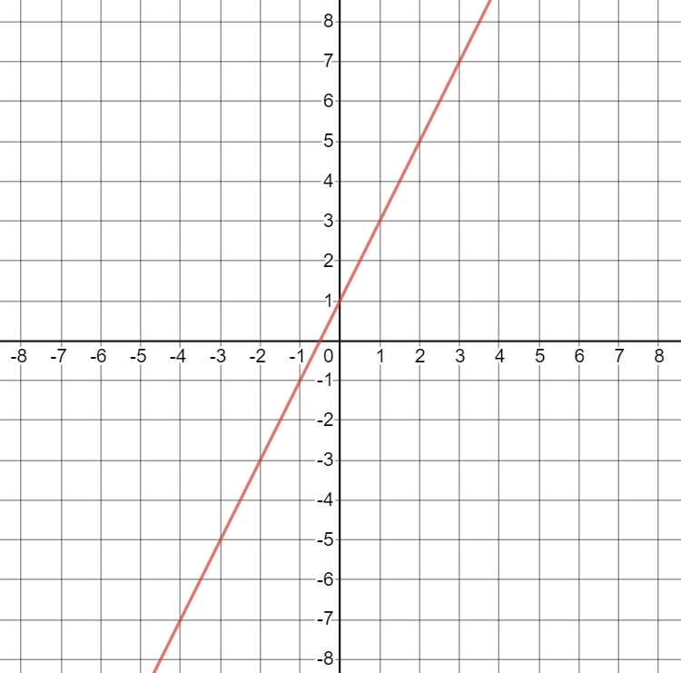
Here are some facts about the equation $y = 2x+1$:

When $x=3$, $y=7$. You can figure this out in two ways:
1. Plug 3 in for x in the equation: $y = 2(3)+1 = 6+1=7$.
2. Find 3 on the x (horizontal) axis in the graph. Draw a vertical line up from $x=3$ on the x-axis to the line. Then, draw a horizontal line to the y (vertical) axis on the left. This line will hit the y-axis at 7.
Now let’s increase $x$ by 1, such that $x=4$. Then $y=9$.
When we increased $x$ by 1, $y$ increased by 2.²⁴ So, for this equation, $m=2$.
When $x=0$, $y=1$. So, for this equation, $b=1$.

Most importantly, when we describe the relationship between $y$ and $x$ above, we phrase it like this: For every one unit increase in x, y increases by 2. During your time in this course, you will be starting many sentences with the magic words “For every one unit increase…” It is important for you to remember these five magic words.

Another way to write a linear equation is like this:

\[ y = b_1x + b_0 \]

In the linear equation above:

$b_1$ = slope
$b_0$ = intercept
$y$ is the dependent variable, the outcome we care about
$x$ is the independent variable, the input that is associated with the dependent variable

Statistical results and formulas are often written with these $b_{something}$ coefficients rather than $m$ and $b$.

Below, we will make an analogy between the linear equations above and a trend line that can be drawn to fit a set of data.

1.5.2 Linear relationship between variables

Linear equations allow us to figure out the relationship between two variables in a data set. That relationship between two variables can be expressed using the same type of linear equation we just reviewed. Before we do that, let’s set up an example. We will look at the mtcars dataset, which is built into R. You can get more information about the mtcars dataset by running the code ?mtcars on your computer. You can also inspect the data by running the code View(mtcars) on your computer.

The mtcars dataset is also displayed below:

mtcars

##                      mpg cyl  disp  hp drat    wt  qsec vs am gear carb
## Mazda RX4           21.0   6 160.0 110 3.90 2.620 16.46  0  1    4    4
## Mazda RX4 Wag       21.0   6 160.0 110 3.90 2.875 17.02  0  1    4    4
## Datsun 710          22.8   4 108.0  93 3.85 2.320 18.61  1  1    4    1
## Hornet 4 Drive      21.4   6 258.0 110 3.08 3.215 19.44  1  0    3    1
## Hornet Sportabout   18.7   8 360.0 175 3.15 3.440 17.02  0  0    3    2
## Valiant             18.1   6 225.0 105 2.76 3.460 20.22  1  0    3    1
## Duster 360          14.3   8 360.0 245 3.21 3.570 15.84  0  0    3    4
## Merc 240D           24.4   4 146.7  62 3.69 3.190 20.00  1  0    4    2
## Merc 230            22.8   4 140.8  95 3.92 3.150 22.90  1  0    4    2
## Merc 280            19.2   6 167.6 123 3.92 3.440 18.30  1  0    4    4
## Merc 280C           17.8   6 167.6 123 3.92 3.440 18.90  1  0    4    4
## Merc 450SE          16.4   8 275.8 180 3.07 4.070 17.40  0  0    3    3
## Merc 450SL          17.3   8 275.8 180 3.07 3.730 17.60  0  0    3    3
## Merc 450SLC         15.2   8 275.8 180 3.07 3.780 18.00  0  0    3    3
## Cadillac Fleetwood  10.4   8 472.0 205 2.93 5.250 17.98  0  0    3    4
## Lincoln Continental 10.4   8 460.0 215 3.00 5.424 17.82  0  0    3    4
## Chrysler Imperial   14.7   8 440.0 230 3.23 5.345 17.42  0  0    3    4
## Fiat 128            32.4   4  78.7  66 4.08 2.200 19.47  1  1    4    1
## Honda Civic         30.4   4  75.7  52 4.93 1.615 18.52  1  1    4    2
## Toyota Corolla      33.9   4  71.1  65 4.22 1.835 19.90  1  1    4    1
## Toyota Corona       21.5   4 120.1  97 3.70 2.465 20.01  1  0    3    1
## Dodge Challenger    15.5   8 318.0 150 2.76 3.520 16.87  0  0    3    2
## AMC Javelin         15.2   8 304.0 150 3.15 3.435 17.30  0  0    3    2
## Camaro Z28          13.3   8 350.0 245 3.73 3.840 15.41  0  0    3    4
## Pontiac Firebird    19.2   8 400.0 175 3.08 3.845 17.05  0  0    3    2
## Fiat X1-9           27.3   4  79.0  66 4.08 1.935 18.90  1  1    4    1
## Porsche 914-2       26.0   4 120.3  91 4.43 2.140 16.70  0  1    5    2
## Lotus Europa        30.4   4  95.1 113 3.77 1.513 16.90  1  1    5    2
## Ford Pantera L      15.8   8 351.0 264 4.22 3.170 14.50  0  1    5    4
## Ferrari Dino        19.7   6 145.0 175 3.62 2.770 15.50  0  1    5    6
## Maserati Bora       15.0   8 301.0 335 3.54 3.570 14.60  0  1    5    8
## Volvo 142E          21.4   4 121.0 109 4.11 2.780 18.60  1  1    4    2

Survey data are arranged in a spreadsheet format, with each row corresponding to an observation and each column corresponding to a characteristic or variable. In this case, the unit of observation is the car, so each row in this data is a car. There are 32 cars in total in the data. A survey-taker surveyed these 32 cars and found out a number of characteristics about them.

Consider this research question: Is a car’s gas efficiency influenced by the number of cylinders it has?

This question is very hard to answer, because we are asking if a car’s cylinders cause its gas efficiency. This question is too hard to answer right now, so we are going to tackle a slightly easier research question: Is gas efficiency, as measured by miles per gallon (mpg) associated with the number of cylinders (cyl) that a car has?

Now it’s time to see what the statistical relationship is between mpg and cyl, or mpg vs cyl, we could say. We always write [dependent variable] vs [independent variable]. Let’s start with a simple scatterplot:

plot(mtcars$cyl,mtcars$mpg, main = "Scatterplot")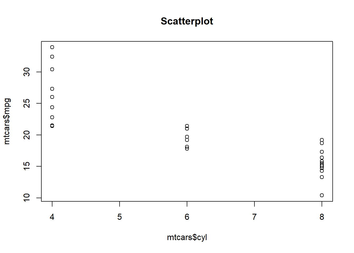

We always put the dependent variable on the y-axis (the vertical axis) and the independent variable on the x-axis (the horizontal axis). Clearly, this plot suggests that there is a noteworthy relationship between mpg and cyl.

Next, we run a linear regression to fit a trend line to this data. At this point in the course, it is not necessary for you to know what exactly a linear regression is. All you need to know for now is that it helped us fit a trend line to the data in our scatterplot above.

Let’s have a look at the scatterplot of our data again, this time including the linear regression trendline:

plot(mtcars$cyl,mtcars$mpg, main = "Scatterplot with trendline")
abline(lm(mpg~cyl,data=mtcars))

This is where we return to the linear equation. The equation of the trendline is:

\[y = -2.9x+37.9\]

In this example, the variables $y$ and $x$ have names other than just $y$ and $x$. Let’s rewrite the equation with these new names:

\[mpg = -2.9cyl+37.9\]

In this case, $y$ is the dependent variable, which is mpg. $x$ is the independent variable, which is cyl. $b_1 = -2.9$ and $b_0 = 37.9$. $b_1$ is the slope and $b_0$ is the intercept.

This is how we phrase the results of this regression analysis: For each additional cylinder, a car is predicted to have 2.9 fewer miles per gallon of gas efficiency. It is not a certainty. It is just a prediction.

We will be interpreting different types of linear equations throughout this course. As we do that, just keep in mind that we are just using slopes to express relationships between dependent and independent variables, the same way we were in the equations and trends that we reviewed above.

1.6 Terminology – selected ambiguities

As you continue your study of quantitative analysis, you will notice that we sometimes use terms interchangeably. For example, the words dataset, spreadsheet, and data frame all mean the same thing. In case this is confusing, the list below might help. It is not necessary for you to understand all of these terms right away. Rather, you can refer back to this list as needed.

List of terms that mean the same thing as each other:

dataset, data set, spreadsheet, dataframe, data frame – A collection of data, formatted like a spreadsheet. You can run View(mtcars) in R on your computer to see an example of this. Also, note that a data.frame is a type of object in R that stores datasets for us. In this textbook, we will use data.frame objects in R to store and interact with our data.
observation, subject, row, data point – A collection of measurements related to a single unit or item that is being studied. These measurements are typically all stored within a single horizontal row of a data spreadsheet.
variable, column, quantitatively measured construct – Attributes that are measured on each observation, typically stored in vertical columns of a data spreadsheet. The names of the variables are typically stored in the topmost row of the data spreadsheet.
coefficient, estimate, slope – When we run a regression model, we get numeric results for each independent variable included in that regression model. One such number tells us the relationship between the dependent variable and a single independent variable. This particular number can be referred to as a coefficient, estimate, or slope.
intercept, constant – Where a regression line or equation intercepts the y-axis. More precisely, the predicted value of the dependent variable when all independent variables are equal to 0.
regression model, regression result, regression equation – These terms all describe the average relationships between a dependent variable and one or more independent variables, as calculated by a regression analysis procedure (such as OLS linear regression, logistic regression, or others).
p-value, p, significance level – The probability that rejecting the null hypothesis in a hypothesis test is a mistake. The probability that the alternate hypothesis was observed due to random chance (rather than because it is the truth).
independent variables, IVs, X variables, the X’s, predictors, covariates, explanatory variables, regressors – The measured quantities that we want to use to predict an outcome of interest.
dependent variable, DV, Y variable, outcome of interest, response variable, regressand – The measured quantity that we want to predict or model based on the independent variables.
predicted value, fitted value – These terms both mean the same thing, meaning the guess that a statistical model makes about the value of the dependent variable for a particular observation.
number of observations, sample size, n – These terms all refer to the number of rows that are in a dataset.
controlling for a variable, holding a variable constant, compare similar observations – These terms all refer to how a regression analysis or matching procedure help us see the relationship between our dependent variable and each independent variable (meaning how the dependent variable is predicted to change for every one unit increase in the independent variable) while all of the other independent variables do not change. This concept is used throughout our study of regression analysis and is also specifically discussed mid-way through the book.

Once again, it is not necessary for you to understand all of the terms above at this early stage in your study of quantitative methods.

You have now reached the end of this week’s content. Please proceed to the assignment below.

1.7 Assignment

This and all future assignments are broken up into multiple sections. Please complete all tasks in all sections and submit them to the instructors. You will turn in all R code that you write in an R script file. You will turn in any other work you do in whatever format you prefer. It is fine for you to submit multiple files in D2L (meaning that you do not need to put all assignment responses into a single file).

In this and all future assignments, you will be given a dataset to use to complete a series of tasks. With instructor permission, you are allowed and encouraged to use a dataset of your own instead of the one supplied in each assignment. If you have some data that is organized in spreadsheet format that you would like to analyze, the assignments in this course are a great way to do that. Talk to an instructor about this as soon as possible!

In this assignment, you will practice handling and manipulating data in R. Then, you will answer some questions about linear equations and relationships.

The deadline for submitting this and future assignments can be found in the course calendar.

1.7.1 Handling and manipulating data in R

To complete this part of the assignment, you should copy lines of code from earlier in this chapter and paste them in a brand new, empty R script file. You will then modify these copied and pasted lines of code to accomplish the tasks below. You will then submit a copy of your R script file (which will of course contain the modifications you made to the code in this chapter after you copied and pasted).

This portion of the assignment will use a single dataset that you will download to your computer. Click here to download the data in an Excel file.²⁵ The data will be in a zipped folder. Move the Excel file to your working directory on your computer. In Excel or another spreadsheet software, open the Excel file and browse through it for a minute or two. It is a dataset about workplace incidents. The dataset is in the SafetyData sheet within the Excel file. In the SafetyData sheet within Excel, remove all spaces from the variable names (in row 1) and then save your work.²⁶

Now that you have downloaded and prepared the Excel file, you are ready to begin!

Task 1: Set the working directory. Put a line of code in your R script file that accomplishes this. Then run that line of code to make sure it works. Once this task is complete, make a new line in your code file and move to the next task!

Task 2: Check to see what the working directory is. Again, you will put the code that accomplishes this task into its own line in your R script file. Please put the code for each task in its own line and run it, even though I won’t remind you to do that anymore!

Task 3: Load the workplace safety data into R. Name the dataset w.

Important note: You should ALWAYS use the code earlier in this chapter (or similar code) to load Excel files. Do NOT use the File -> Import Dataset tool in RStudio and do NOT use any other point-and-click options you might see to import your data into R, because this will give you trouble later on when you are trying to replicate your work or re-run your entire analysis at once.

Task 4: View your dataset w as a spreadsheet in RStudio to make sure it was loaded correctly.

Task 5: How many observations are in the data?

Task 6: How many variables are in the data?

Task 7: Write a line of code to display the names of all variables in the data.

Task 8: How many qualitative/categorical variables are in the data? What are the names of these variables?

Task 9: How many numeric variables are in the data? What are the names of these variables?

Task 10: Make a one-way table to figure out how many women and how many men are in the dataset.

Task 11: Make a two-way table to look at the distribution of incidents involving men and women across different report types.

Task 12: Create a subset of w, called wburns, which contains only incidents that involved burns. Remember that it may be useful to look at your data as a spreadsheet—either in Excel or RStudio—as you figure this out!

Task 13: In wburns, create a new version of the Shift variable, called ShiftBinary. The table below will tell you what exactly to recode. Make a two-way table to check if your recode was successful.

Old Shift variable	New ShiftBinary variable
Day	Light
Afternoon	Light
Night	Dark

Task 14: In w, Recode the IncidentCost variable into a new variable called CostBinary such that incidents costing less than or equal to 2500 are labeled as Low and costs over 2500 are labeled as High. Make a one-way table of CostBinary to see how many low and high cost incidents there are.

Task 15: Create a new variable in w called DaysLostSq which is the square of the variable DaysLost.

Task 16: As far as you can tell, what is the unit of observation in the workplace incidents data (w)?

1.7.2 Linear relationships

Now we will turn to a review of linear relationships. Some of the tasks below relate to datasets that you have encountered earlier in this chapter and others relate more conceptually to linear relationships.

You can write down your answers anywhere you would like and then submit them as a separate file in D2L. For example, you can write your answers to this part of the assignment in a Microsoft Word document. Then, you would submit both the Word document and your R script file from above (two files total) in D2L. You could also do this part of the assignment on paper and then scan/photograph your work to submit.

Task 17: Draw a small coordinate plane (graph) on a paper. Graph the line represented by the equation $y = -1.5x+5$. When $x = 2$, what is $y$? Plug 2 into the equation in place of x to figure it out! Show all of your work. Please feel free to do this on paper and then scan/photograph your work for us to see.

Task 18: In the same equation, $y = -1.5x+5$, what is $y$ when $x=3$?

Task 19: For the equation $y = -1.5x+5$, how do you express the relationship between $y$ and $x$? Make sure your answer begins with the five magic words “For every one unit increase…”²⁷

Task 20: In the equation $y = -1.5x+5$, what is the dependent variable and what is the independent variable?

Task 21: Earlier in the chapter, we found that the predicted relationship between mpg and cyl in the mtcars data is described by the equation $mpg = -2.9cyl+37.9$. In this equation, what is the dependent variable and what is the independent variable?

Task 22: Based on the equation $mpg = -2.9cyl+37.9$, if a car has 4 cylinders, what is its predicted fuel efficiency? Show each step of your work.

Task 23: Based on the equation $mpg = -2.9cyl+37.9$, if a car has 3 cylinders, what is its predicted fuel efficiency? Show your work.

Task 24: What is the difference in predicted mpg for a car with 4 cylinders compared to a car with 3 cylinders? What is another name for this difference, in the terminology of linear equations?

Task 25: Interpret the number -2.9 from the equation $mpg = -2.9cyl+37.9$. Be sure to use the five magic words as part of your answer!

1.7.3 Follow up and submission

You have now reached the end of this week’s assignment. The tasks below will guide you through submission of the assignment and allow us to gather questions and/or feedback from you.

Task 26: Please write any questions you have for the course instructors (optional).

Task 27: Please write any feedback you have about the instructional materials (optional).

Task 28: Please submit your assignment (multiple files are fine) to the D2L assignment drop-box corresponding to this chapter and week of the course. To get to the drop-box, go to the D2L page for this course, click on Assessments -> Assignments. Please e-mail all instructors if you experience any difficulty with this process.

There may be exceptions to this guideline depending on what exactly you use RStudio for, but in general this is likely the right thing to say.↩︎
Data source: Excel Sample Data. Contextures. https://www.contextures.com/xlsampledata01.html.↩︎
These two arguments are separated by a comma.↩︎
You may have noticed that the numbers in these tables contain an unnecessary number of decimal places, making the table a bit unpleasant to look at. If you want to fix this, one change you can make is to put all of the code we used—prop.table(table(dat$Category))*100—into the round(...) function, like this: round(prop.table(table(dat$Category))*100,1). In this code, the number 1 is telling the computer how many decimal places we want to include. More precisely: we are inserting two arguments into the round(...) function, separated by commas: 1) prop.table(table(dat$Category))*100 – this is the object (a table in this case) that we want to round; 2) 1 – this is the number of decimal places to which we want to round the object given in the first argument (try changing this to 0 or any other number and see what happens).↩︎
Source: Subsetting Data. https://www.statmethods.net/management/subset.html.↩︎
Remember, in other examples that you may have encountered so far, the name of this dataset may have been d, dat, or even something else!↩︎
Adapted from: Operators. Quick-R by datacamp. https://www.statmethods.net/management/operators.html.↩︎
This is a simplified version of what the %>% operator—called the pipe operator—technically does for us. ↩︎
We could call it whatever we want. I’m calling it this because it’s now a binary variable with just two possible values.↩︎
A vector is denoted by the c(...) notation.↩︎
Adapted from the answer by Rahul at https://stats.stackexchange.com/questions/6759/removing-duplicated-rows-data-frame-in-r. Accessed on April 28 2020.↩︎
Produced using the graphing calculator at https://www.desmos.com/calculator.↩︎
Remember: when x was 3, y was 7. When we increased x to 4, y became 9. y changed from 7 to 9, which means that it increased by 2 when we increased x by 1.↩︎
Data source: Excel Sample Data. Contextures. https://www.contextures.com/xlsampledata01.html.↩︎
For example, one of the variables is called Report Type. Please change this to ReportType, with no space in between the words “Report” and “Type.”↩︎
Hint: Look at your answers to the previous two quesions. What was the value of y when x was 2? What was the new value of y when you changed x to 3? What is the difference between these two values of y? That difference is the change in y for every one-unit change in x.↩︎