Chapter 13 Missing Data

This week, our goals are to…

Identify situations that lead to missing data in health professions education data.
Explore different strategies for imputing missing data.
Use and compare three strategies to compensate for missing data.

Announcements and reminders

The course evaluation for HE902 is now available online (or will be soon). You will receive an email about it through MGHIHP. Please fill this out when you have a chance so that your feedback can be incorporated into future offerings of the course.
If you have not done so already, please email Nicole and Anshul to schedule a time for your Oral Exam #3.

13.1 Define Missing Data

Previously in this textbook, any time we have encountered datasets with missing data, we have deleted all of the rows in our dataset that contain missing data. This is called list-wise deletion. This week, we will learn about options other than list-wise deletion for dealing with missing data. We will learn ways to fill in missing data, using the other data in our dataset to predict any missing values.

In this chapter, you will see examples of how missing data techniques can be applied in R. Then, in your assignment, you will practice using at least one of these techniques on different versions of the same dataset, to see how different proportions of missing data vary with our ability to estimate regression coefficients.

The following extended quotation from Chaitanya Sagar²⁰⁹ is an excellent introduction to missing data:

Missing Data in Analysis

At times while working on data, one may come across missing values which can potentially lead a model astray. Handling missing values is one of the worst nightmares a data analyst dreams of. If the dataset is very large and the number of missing values in the data are very small (typically less than 5% as the case may be), the values can be ignored and analysis can be performed on the rest of the data. Sometimes, the number of values are too large. However, in situations, a wise analyst ‘imputes’ the missing values instead of dropping them from the data.

What Are Missing Values

Think of a scenario when you are collecting a survey data where volunteers fill their personal details in a form. For someone who is married, one’s marital status will be ‘married’ and one will be able to fill the name of one’s spouse and children (if any). For those who are unmarried, their marital status will be ‘unmarried’ or ‘single’.

At this point the name of their spouse and children will be missing values because they will leave those fields blank. This is just one genuine case. There can be cases as simple as someone simply forgetting to note down values in the relevant fields or as complex as wrong values filled in (such as a name in place of date of birth or negative age). There are so many types of missing values that we first need to find out which class of missing values we are dealing with.

Types of Missing Values

Missing values are typically classified into three types - MCAR, MAR, and NMAR.

MCAR stands for Missing Completely At Random and is the rarest type of missing values when there is no cause to the missingness. In other words, the missing values are unrelated to any feature, just as the name suggests.

MAR stands for Missing At Random and implies that the values which are missing can be completely explained by the data we already have. For example, there may be a case that Males are less likely to fill a survey related to depression regardless of how depressed they are. Categorizing missing values as MAR actually comes from making an assumption about the data and there is no way to prove whether the missing values are MAR. Whenever the missing values are categorized as MAR or MCAR and are too large in number then they can be safely ignored.

If the missing values are not MAR or MCAR then they fall into the third category of missing values known as Not Missing At Random, otherwise abbreviated as NMAR. The first example being talked about here is NMAR category of data. The fact that a person’s spouse name is missing can mean that the person is either not married or the person did not fill the name willingly. Thus, the value is missing not out of randomness and we may or may not know which case the person lies in. Who knows, the marital status of the person may also be missing!

If the analyst makes the mistake of ignoring all the data with spouse name missing he may end up analyzing only on data containing married people and lead to insights which are not completely useful as they do not represent the entire population. Hence, NMAR values necessarily need to be dealt with.

Imputing Missing Values

Data without missing values can be summarized by some statistical measures such as mean and variance. Hence, one of the easiest ways to fill or ‘impute’ missing values is to fill them in such a way that some of these measures do not change. For numerical data, one can impute with the mean of the data so that the overall mean does not change.

In this process, however, the variance decreases and changes. In some cases such as in time series, one takes a moving window and replaces missing values with the mean of all existing values in that window. This method is also known as method of moving averages.

For non-numerical data, ‘imputing’ with mode is a common choice. Had we predict the likely value for non-numerical data, we will naturally predict the value which occurs most of the time (which is the mode) and is simple to impute.

In some cases, the values are imputed with zeros or very large values so that they can be differentiated from the rest of the data. Similarly, imputing a missing value with something that falls outside the range of values is also a choice.

An example for this will be imputing age with -1 so that it can be treated separately. However, these are used just for quick analysis. For models which are meant to generate business insights, missing values need to be taken care of in reasonable ways. This will also help one in filling with more reasonable data to train models.

Now that you have read the short primer above, which was quoted from Chaitanya Sagar,²¹⁰ continue reading to see an example and begin our exploration of how to deal with missing data!

13.2 Example Study

In this chapter, we will refer to an example to demonstrate multiple missing data techniques. For this example, we will use the diabetes.sav dataset. You can click here to download the dataset.

Then run the following code to load the data into R, so that you can follow along:

if (!require(foreign)) install.packages('foreign')
library(foreign)

diabetes <- read.spss("diabetes.sav", to.data.frame = TRUE)

Our research question of interest is:

What is the relationship between total cholesterol and age, controlling for weight and gender?

These are the variables we will use:

Dependent variable: total_cholesterol
Independent variables: weight, age, gender

We will use an ordinary least squares (OLS) linear regression throughout this chapter. However, keep in mind that all of the techniques in this chapter could possibly be used on any type of study with any type of regression model.

Let’s continue to prepare the data for use throughout this chapter.

We will extract only the variables that we plan to use:

if (!require(dplyr)) install.packages('dplyr')
library(dplyr)

d <- diabetes %>%
  dplyr::select(total_cholesterol, age, gender, weight)

Now the name of our dataset is d and it only contains the variables that we will use in this example. Here are the variables remaining in the data:

names(d)

## [1] "total_cholesterol" "age"               "gender"           
## [4] "weight"

This dataset does not have much missing data. However, since this week’s topic is about missing data, we actually need to remove some of the data from our dataset. We will randomly remove 30% of the data from d, using the following code:

if (!require(missForest)) install.packages('missForest')
library(missForest)

d.na <- prodNA(d, noNA = 0.3)

Above, we did the following:

Load the package missForest, which contains the function prodNA()
Use the prodNA() function to create a new dataset called d.na which is a copy of the dataset d but with a proportion of 0.3 (30%) of the data randomly removed.

If you were adapting this code for your own use, you would make the following changes:

Change d.na to whatever name you would want your new dataset to have (the dataset with some missing data).
Change d to your input dataset, the old dataset from which you want to remove some values.
Change 0.3 to the proportion of missing data that you wish to randomly remove.

In our two datasets, d and d.na, each has 403 observations (rows of data, which in this case means number of people in the data). We can confirm this by running the following two commands:

nrow(d)

## [1] 403

nrow(d.na)

## [1] 403

As you can see above, R tells us that both datasets have 403 observations each.

Now that we have created a pretend dataset with some missing values, continue reading to see how we can inspect the data and then figure out what to do about it.

13.3 Inspect Missing Data

In this section, we will review two ways to learn about the nature of any missing data in our datasets. The first technique is visual inspection and the second technique is using the mice package.

13.3.1 Visual Inspection

Continuing with our example from the diabetes dataset earlier in this chapter, it is time to inspect our data visually. This simply means that we will look at our data in tabular form to see which data missing. Nothing fancy.

Remember that we now have two datasets:

d is a dataset which is just the diabetes dataset but the variables we aren’t interested in have been removed.
d.na is a copy of d, but 30% of the data has been randomly removed, so there is a lot of data missing in the dataset d.na.

Comparing d and d.na allows us to understand how a regression analysis might differ in the two scenarios. With d, we are pretending that we have conducted a study with nearly complete data. With d.na, we are imagining that we did the very same study but there was a bunch of missing data. In the future, you might find yourself in either of these situations as a researcher, which is why we are comparing the two situations in this chapter.

Let’s look at the first ten rows of the original dataset, d:

head(d, n=10)

##    total_cholesterol age gender weight
## 1                203  46 female    121
## 2                165  29 female    218
## 3                228  58 female    256
## 4                 78  67   male    119
## 5                249  64   male    183
## 6                248  34   male    190
## 7                195  30   male    191
## 8                227  37   male    170
## 9                177  45   male    166
## 10               263  55 female    202

As we can see above, all of the data is complete for the first ten people in this dataset. We know everybody’s total cholesterol, age, gender, and weight.

Below are the first ten rows of d.na, which is a copy of d in which 30% of the data has been randomly removed:

head(d.na,n=10)

##    total_cholesterol age gender weight
## 1                203  46 female    121
## 2                165  29 female     NA
## 3                228  58 female    256
## 4                 78  67   <NA>     NA
## 5                249  NA   <NA>    183
## 6                248  34   male     NA
## 7                 NA  30   male    191
## 8                227  37   male    170
## 9                177  NA   male    166
## 10               263  55   <NA>    202

As you can see, there are many missing values in d.na above. Missing values are indicated where you see NA written instead of a number. In R, NA is treated as a number that is unknown. Therefore, NA can still appear in numeric data even though we are using characters to indicate a missing value.

Above, we visually inspected our data tables to understand which data is present and which data is missing, in both our d and d.na datasets.

13.3.2 `mice` Package

In this section, we will once again inspect both our d and d.na datasets using tools available to us in the mice package in R. MICE stands for Multivariate Imputation by Chained Equations. As this title foreshadows, we will be using it later in this chapter to impute missing values in our data. But we’ll get to that in a little while. First we need to finish inspecting our data.

Let’s install and load the mice package:

if (!require(mice)) install.packages('mice')
library(mice)

13.3.2.1 Missing Data Pattern Report

Next, let’s have the md.pattern() function give us a report about the missing data in the dataset d.na:

md.pattern(d.na)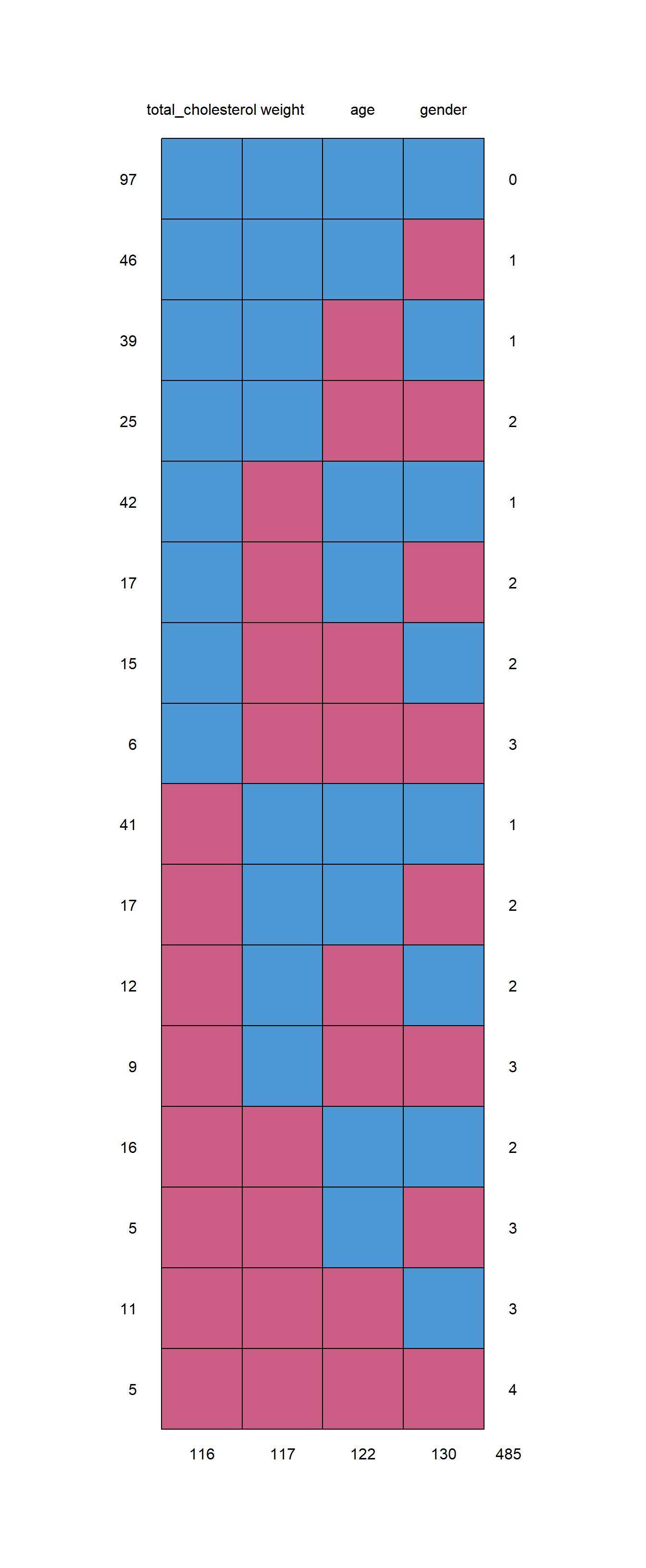

##    total_cholesterol weight age gender    
## 97                 1      1   1      1   0
## 46                 1      1   1      0   1
## 39                 1      1   0      1   1
## 25                 1      1   0      0   2
## 42                 1      0   1      1   1
## 17                 1      0   1      0   2
## 15                 1      0   0      1   2
## 6                  1      0   0      0   3
## 41                 0      1   1      1   1
## 17                 0      1   1      0   2
## 12                 0      1   0      1   2
## 9                  0      1   0      0   3
## 16                 0      0   1      1   2
## 5                  0      0   1      0   3
## 11                 0      0   0      1   3
## 5                  0      0   0      0   4
##                  116    117 122    130 485

The report above (in both tabular and graphical format) tells us all of the patterns of missing data in our dataset d.na and counts all of them. I prefer to look at the table but you can look at whichever one you prefer!

Here are some features of this report:

There is one column for each variable.
Each row is a pattern of missing data, with 0 indicating missing data for a given variable and 1 indicated no missing data for that variable.
The first column is a count of how often each pattern occurs in the data.
The final column is a count of how many variables have missing data in a given pattern (row).
The final row tells us total numbers of observations that have missing data for each variable.

Example interpretation:

In the top-most row, we see that there are 97 people/observations (rows of data) in d.na that do not have any missing data. This is because there is a 1 for all four variables. At the end of this row, we see the number 0, because in this pattern of missing data—for these 97 rows in our data—there are zero variables for which we have missing data.
In the sixth row of the report, we see that there are 17 observations in our data d.na for which total_cholesterol and age are present (since they are marked with 1 in that row of the report), while weight and gender are missing (because they are marked with 0 in that row of the report).
In the final row of the report, we see that there are 116 observations (rows) in which total_cholesterol is missing. This means that in 116 out of a total of 403 observations in d.na, there is no value for total_cholesterol. Likewise, there are 117, 122, and 130 observations with missing values for weight, age, and gender respectively.

Before we move on, let’s quickly run the same report for d, the original diabetes dataset without 30% of the data removed. We will use the same code as above, but put d where d.na used to be:

md.pattern(d)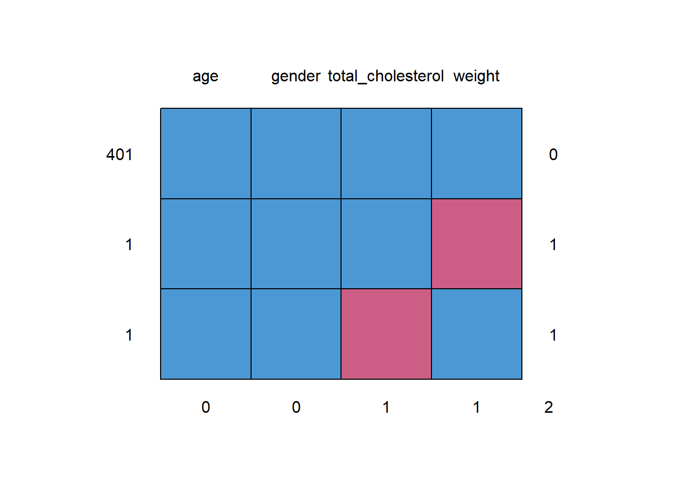

##     age gender total_cholesterol weight  
## 401   1      1                 1      1 0
## 1     1      1                 1      0 1
## 1     1      1                 0      1 1
##       0      0                 1      1 2

The table shows that for 401 of the 403 observations, the data is complete. All four variables have a 1 in the first row. Then, there is one observation for which weight is missing and another for which total cholesterol is missing. The corresponding plot also shows the same thing.

13.3.2.2 Missing Data Pairs Report

The previous report told us the prevalence of each pattern of missing values in our dataset. Now we will see another type of report that focuses on the pairs of variables in our dataset.

Imagine that if our dataset has variables A and B in it, there are four scenarios possible in each row with respect to A and B:²¹¹

both A and B are observed (pattern rr);

A is observed and B is missing (pattern rm);

A is missing and B is observed (pattern mr);

both A and B are missing (pattern mm).

I think it is easier to look at an example rather than further explain this.

We can generate a pairs report with the following code that uses the md.pairs() function that is also in the mice package:

md.pairs(d.na)

## $rr
##                   total_cholesterol age gender weight
## total_cholesterol               287 202    193    207
## age                             202 281    196    201
## gender                          193 196    273    189
## weight                          207 201    189    286
## 
## $rm
##                   total_cholesterol age gender weight
## total_cholesterol                 0  85     94     80
## age                              79   0     85     80
## gender                           80  77      0     84
## weight                           79  85     97      0
## 
## $mr
##                   total_cholesterol age gender weight
## total_cholesterol                 0  79     80     79
## age                              85   0     77     85
## gender                           94  85      0     97
## weight                           80  80     84      0
## 
## $mm
##                   total_cholesterol age gender weight
## total_cholesterol               116  37     36     37
## age                              37 122     45     37
## gender                           36  45    130     33
## weight                           37  37     33    117

Above, we see four tables, each corresponding to one missing data pair pattern in the list displayed earlier. Some examples will help explain this. Let’s consider the variables weight and gender:

The rr table tells us that there are 189 out of 403 observations for which both weight and gender are observed (not missing).
The rm table tells us that there are 97 observations for which weight is observed and gender is not observed.
The mr table tells us that there are 84 observations for which weight is not observed and gender is observed.
The mm table tells us that there are 33 observations for which both weight and gender are not observed (meaning they are missing).

We will not discuss the technicalities of how this table is useful. In some situations, the numbers in this table can give us a sense for how useful each variable is in imputing the other. For example, there are 117 out of 403 observations for which weight is missing. In these 117 instances in which weight is missing, gender is also missing 33 times and gender is observed 84 times. gender is observed in \(\frac{84}{117} * 100=71.8\%\) of the observations in which weight is missing. In addition to this, there are the 189 observations in which both weight and gender are observed (not missing), which will also help us use gender (and other variables) to impute weight later in this chapter.

Now that you have seen a few ways to inspect your dataset to look for missing data patterns, we will conduct some OLS regressions on our example data and turn to the issue of what to do about missing data.

13.4 True Effect – Initial Regression Analysis

As I said earlier in this chapter when introducing the diabetes data, we will try to answer the following research question in this example:

What is the relationship between total cholesterol and age, controlling for weight and gender?

And here, once again, are the variables we will use:

Dependent variable: total_cholesterol
Independent variables: weight, age, gender

Let’s run an OLS regression to get an initial answer to our research question:

summary(reg.true <- lm(total_cholesterol ~ weight + age + gender, data = d))

## 
## Call:
## lm(formula = total_cholesterol ~ weight + age + gender, data = d)
## 
## Residuals:
##      Min       1Q   Median       3Q      Max 
## -136.198  -26.684   -4.697   22.822  225.533 
## 
## Coefficients:
##               Estimate Std. Error t value Pr(>|t|)    
## (Intercept)  158.67383   12.48237  12.712  < 2e-16 ***
## weight         0.09251    0.05380   1.719   0.0863 .  
## age            0.66441    0.13206   5.031 7.41e-07 ***
## genderfemale   3.16853    4.38681   0.722   0.4705    
## ---
## Signif. codes:  0 '***' 0.001 '**' 0.01 '*' 0.05 '.' 0.1 ' ' 1
## 
## Residual standard error: 42.97 on 397 degrees of freedom
##   (2 observations deleted due to missingness)
## Multiple R-squared:  0.06438,    Adjusted R-squared:  0.05731 
## F-statistic: 9.107 on 3 and 397 DF,  p-value: 7.663e-06

Above, we see that there is a predicted increase in total cholesterol of 0.66 units for every one year increase in age, controlling for weight and gender. It has a very low p-value, which tells us that we can be extremely confident about this estimate, if all of the assumptions of OLS linear regression are true for this model.

Since we used the dataset d—which is the full original dataset—in the regression above, let’s call 0.66 the true effect (or true association or relationship) of age on total cholesterol.

In the rest of this chapter, we will use the other dataset, d.na—which is a version of d that has 30% of the data randomly removed—to see if we can still use it to calculate the true effect of 0.66 that we found above. The next section describes and demonstrates strategies we can use to use a dataset with missing data to still answer our research question using regression analysis.

13.5 Addressing Missing Data

In this section, we will address multiple approaches that can be used to compensate for missing data in a dataset. These include deletion, mean imputation, and multiple imputation with the mice package. As we have been doing throughout this chapter, we will use the datasets d and d.na that we created earlier to go through all of these approaches.

Remember, we created d.na to see what it would be like to do a research project in which 30% of our data is unobserved. In this case, we happen to also have d, in which almost all of the data is observed.

After reading this section, you may still be wondering which of the presented approaches is the best one to use. There is no one right answer to the question. It depends on the project, how much missing data is there, and why that data is missing. I typically recommend that you try to use multiple of the approaches below and see if the results you get are the same each time or different. If they are the same, that can often be a sign that you can be more definite about the answer to your research question. If they are different, then you may need to delve into the assumptions and calculation techniques of each method to figure out which one is most appropriate for your situation.

13.5.1 Deletion

The first strategy for addressing missing data is to simply delete observations that have missing values for one or more variables. This is called listwise deletion. We have actually been doing this throughout this semester when running regressions. This is the default way that R handles missing data when we run a regression command. It is also what happens when we use the na.omit() command that we have used before to prepare our data.

To fully understand listwise deletion, let’s again look at the first ten rows of the d.na dataset:

head(d.na,n=10)

##    total_cholesterol age gender weight
## 1                203  46 female    121
## 2                165  29 female     NA
## 3                228  58 female    256
## 4                 78  67   <NA>     NA
## 5                249  NA   <NA>    183
## 6                248  34   male     NA
## 7                 NA  30   male    191
## 8                227  37   male    170
## 9                177  NA   male    166
## 10               263  55   <NA>    202

If we were to do listwise deletion on these first 10 rows, observations #2, 4, 5, 6, 7, 9, and 10 would all be removed because each of them has at least one missing value in it. We saw earlier that out of the 403 observations in d.na, 97 were complete and did not have missing data. The remaining 306 observations had values for one or more variables missing.

Earlier, we got the true effect for our research question by doing our regression using the d dataset. Now, we will do the exact same regression on the d.na dataset:

summary(reg.del <- lm(total_cholesterol ~ weight + age + gender, data = d.na))

## 
## Call:
## lm(formula = total_cholesterol ~ weight + age + gender, data = d.na)
## 
## Residuals:
##     Min      1Q  Median      3Q     Max 
## -85.038 -25.390  -5.243  11.590 121.653 
## 
## Coefficients:
##               Estimate Std. Error t value Pr(>|t|)    
## (Intercept)  184.43803   24.11122   7.649 1.82e-11 ***
## weight         0.14438    0.09692   1.490    0.140    
## age            0.20047    0.27273   0.735    0.464    
## genderfemale -10.03657    8.76972  -1.144    0.255    
## ---
## Signif. codes:  0 '***' 0.001 '**' 0.01 '*' 0.05 '.' 0.1 ' ' 1
## 
## Residual standard error: 42.49 on 93 degrees of freedom
##   (306 observations deleted due to missingness)
## Multiple R-squared:  0.04273,    Adjusted R-squared:  0.01186 
## F-statistic: 1.384 on 3 and 93 DF,  p-value: 0.2526

The output above tells us that 306 observations were deleted due to missing data, as we predicted earlier. Let’s confirm how many observations were used in the regression above:

nobs(reg.del)

## [1] 97

Above, the computer has confirmed that 97 observations were indeed used in this analysis.

Let’s see what the answer to our research question would be if we just used this regression with 97 observations. The regression predicts an increase in total cholesterol of 0.2 for each one-unit increase in age, holding constant weight and gender. However, this estimate has a very high p-value, meaning that we cannot be confident at all about the estimated effect of 0.2. So, using listwise deletion gave us an incorrect estimate of the true effect (which was 0.66 units of cholesterol).

13.5.1.1 Suggested deletion procedure

Sometimes you may want to use listwise deletion to remove missing values before you do a procedure such as a regression. Below is a quick way that you can remove missing data in a quick—though not necessarily the best—way so that you can run a regression or do another procedure.

First, use the following code make a new dataset that contains ONLY the variables you want to use from your dataset (the one with missing values):²¹²

if (!require(dplyr)) install.packages('dplyr')
library(dplyr)

NewData <- OldData %>%
  dplyr::select(var1, var2, var3)

Now you have a new version of your dataset called NewData which only contains the variables you will use in your analysis (which in the example above are called var1, var2, and var3). This variable-based subsetting procedure was introduced earlier in this textbook.

Next, you can remove all missing data in one single command. This will remove all rows of data in which even one variable has a missing value (which in R is coded as NA):

EvenNewerData <- na.omit(NewData)

And then just use the dataset EvenNewerData for the rest of your analysis (and ignore NewData and OldData)!

If we don’t want to use deletion to deal with our missing data problem, we have to find a way to fill in each missing in our data table. This is where the idea of imputation comes in.

13.5.2 Imputation

Imputation is a word we use to simply mean filling in the missing values. There are different types of strategies we could use. For example, we could fill in all missing values in our dataset d.na with a random number. This would not be particularly reasonable. Another strategy could be to simply take the mean for each variable (calculated with the observations that do not have a missing value for that variable) and plug that in for each observation that has a missing value for that variable. You will see a demonstration of this later in this chapter.

Another idea, though, is to make multiple (more than one) guesses about what each missing value might be in a given cell of our data table. This approach is called multiple imputation.²¹³ This is now a very commonly used strategy for dealing with missing data, and we will examine this method carefully below.

13.5.3 Mean imputation

Before we try anything fancier, let’s simply try to impute all missing values using calculation of mean values. Once again, we are using the dataset d.na in which about 30% of the data is missing. Let’s start by looking at both a summary table and the first ten rows of d.na:

summary(d.na)

##  total_cholesterol      age           gender        weight     
##  Min.   : 78.0     Min.   :19.00   male  :118   Min.   : 99.0  
##  1st Qu.:179.0     1st Qu.:33.00   female:155   1st Qu.:152.2  
##  Median :204.0     Median :44.00   NA's  :130   Median :174.5  
##  Mean   :208.4     Mean   :46.37                Mean   :179.3  
##  3rd Qu.:232.0     3rd Qu.:59.00                3rd Qu.:200.0  
##  Max.   :443.0     Max.   :92.00                Max.   :320.0  
##  NA's   :116       NA's   :122                  NA's   :117

Above, we have the summary of d.na for each variable. Below, we have the first ten rows of d.na. Here is what we learn from the summary above:

The mean of total_cholesterol in our data is 208.4. This is the value we would get if we look at all of the total cholesterol measurements in the data and ignored the missing values. Referring to the table below, we would ignore row #7 where total_cholesterol is missing. We would then calculate the mean of the remaining 9 values. We would do this for all 403 rows of the data, ignoring the missing values and calculating the mean of the total_cholesterol values that remain.
The mean of age is 46.4, when ignoring missing values, as we did for total_cholesterol.
No mean is calculated for gender since it is categorical, again ignoring missing values.
The mean of weight is 179.3, again ignoring missing values.

head(d.na,n=10)

##    total_cholesterol age gender weight
## 1                203  46 female    121
## 2                165  29 female     NA
## 3                228  58 female    256
## 4                 78  67   <NA>     NA
## 5                249  NA   <NA>    183
## 6                248  34   male     NA
## 7                 NA  30   male    191
## 8                227  37   male    170
## 9                177  NA   male    166
## 10               263  55   <NA>    202

Now that we have calculated the means for all variables (based on the non-missing values), our plan is to replace all missing values with the means for the corresponding variable. Let’s refer to the first ten rows of d.na above to see what we mean:

The NA in the total_cholesterol cell for row #7 will be replaced with the mean for total_cholesterol, which is 208.4.
The NA values in rows #5 and 9 for age will both be replaced by the mean of age, which is 46.4.
Rows #4, 5, and 10 will be replaced with the most frequently occurring gender, which is female.
Rows #2, 4, and 6 will be replaced with the mean of weight, which is 179.3.

The following code will make these replacements for us:

d.na.mean <- d.na # make a copy

d.na.mean$total_cholesterol <- ifelse(is.na(d.na$total_cholesterol),mean(d.na$total_cholesterol,na.rm = T),d.na.mean$total_cholesterol)

d.na.mean$age <- ifelse(is.na(d.na$age),mean(d.na$age,na.rm = T),d.na.mean$age)

d.na.mean$weight <- ifelse(is.na(d.na$weight),mean(d.na$weight,na.rm = T),d.na.mean$weight)

d.na.mean[which(is.na(d.na.mean$gender)),]$gender <- "female"

Let’s inspect the first 10 rows of our new dataset, d.na.mean, which is a copy of d.na in which the mean has been inserted for each variable in place of each missing value.

head(d.na.mean,n=10)

##    total_cholesterol      age gender   weight
## 1           203.0000 46.00000 female 121.0000
## 2           165.0000 29.00000 female 179.3147
## 3           228.0000 58.00000 female 256.0000
## 4            78.0000 67.00000 female 179.3147
## 5           249.0000 46.37011 female 183.0000
## 6           248.0000 34.00000   male 179.3147
## 7           208.4077 30.00000   male 191.0000
## 8           227.0000 37.00000   male 170.0000
## 9           177.0000 46.37011   male 166.0000
## 10          263.0000 55.00000 female 202.0000

We have now successfully imputed all of the missing data, replacing each missing value with the mean value of each variable.

Once again, we can run the same OLS regression to answer our research question, this time on our new dataset called d.na.mean:

summary(reg.mean <- lm(total_cholesterol ~ weight + age + gender, data = d.na.mean))

## 
## Call:
## lm(formula = total_cholesterol ~ weight + age + gender, data = d.na.mean)
## 
## Residuals:
##      Min       1Q   Median       3Q      Max 
## -133.039  -18.924   -0.796   11.207  230.891 
## 
## Coefficients:
##               Estimate Std. Error t value Pr(>|t|)    
## (Intercept)  185.24278   12.94519  14.310   <2e-16 ***
## weight         0.09783    0.05668   1.726   0.0851 .  
## age            0.21220    0.13731   1.545   0.1230    
## genderfemale  -5.96394    4.19104  -1.423   0.1555    
## ---
## Signif. codes:  0 '***' 0.001 '**' 0.01 '*' 0.05 '.' 0.1 ' ' 1
## 
## Residual standard error: 38.2 on 399 degrees of freedom
## Multiple R-squared:  0.01862,    Adjusted R-squared:  0.01124 
## F-statistic: 2.523 on 3 and 399 DF,  p-value: 0.05735

Above, we ran the same regression code as before, but we changed the data to d.na.mean (and we of course changed the saved name of the regression model to reg.mean). The estimate of age is 0.21 units of cholesterol, which is very close to the estimate we got when we used deletion. This time, however, the confidence level is higher because the p-value is much lower, at 0.123. Still, it is not a very good estimate of the true effect which we calculated earlier (which was 0.66 units of cholesterol).

Another strategy we can try is multiple imputation, which was defined above. Keep reading to see an example and demonstration of this technique!

13.5.4 Multiple Imputation With MICE

Now we are ready to try multiple imputation. To do this, we will use the mice package. As a reminder, our dataset that we will start with is called d.na, which is a version of the diabetes dataset that has 30% of its data missing. We have already tried using deletion and mean imputation as strategies for resolving our missing data problem. Now we will try the mice package and see if it can do better.

13.5.4.1 `mice` Package Information

Here is a quoted description of the mice package:²¹⁴

The mice package which is an abbreviation for Multivariate Imputations via Chained Equations is one of the fastest and probably a gold standard for imputing values.

The mice package in R is used to impute MAR values only. As the name suggests, mice uses multivariate imputations to estimate the missing values. Using multiple imputations helps in resolving the uncertainty for the missingness.

The package provides four different methods to impute values with the default model being linear regression for continuous variables and logistic regression for categorical variables. The idea is simple!

If any variable contains missing values, the package regresses it over the other variables and predicts the missing values.

13.5.4.2 Running the Imputation

Let’s get started by loading the mice package and running a basic imputation:

if (!require(mice)) install.packages('mice')
library(mice)

d.na.mice <- mice(d.na)

In the code above, we loaded the package mice. Then we created a new object called d.na.mice which is the stored result of the mice() function. The mice function includes d.na as an argument because that’s the dataset for which we want to impute missing data.

Let’s learn a bit more about the d.na.mice stored data object that we created, by running the class() function on it:

class(d.na.mice)

## [1] "mids"

We are told by the output above that d.na.mice is a mids object. mids stands for multiply imputed data set.²¹⁵ d.na.mice is a new dataset that contains five different versions of imputed datasets that were returned by the mice function. We can inspect each of these datasets using the complete() function:

temp <- complete(d.na.mice,1)

Above, we made a new dataset called temp which is the first of five datasets created by our imputation procedure. The complete() function tells the computer that we want to see a complete, imputed dataset. The d.na.mice argument tells the computer that we want to retrieve one of the completely imputed datasets stored in d.na.mice (which we had created above using the mice() function). And the 1 argument says that we want to retrieve the first of the five stored datasets. We could change the 1 argument to any number up to 5 to see the five different imputed datasets (versions of imputations) that have been stored.

Now let’s look at the first ten rows of temp, the first of the imputed datasets:

head(temp,n=10)

##    total_cholesterol age gender weight
## 1                203  46 female    121
## 2                165  29 female    144
## 3                228  58 female    256
## 4                 78  67 female    158
## 5                249  51 female    183
## 6                248  34   male    202
## 7                200  30   male    191
## 8                227  37   male    170
## 9                177  37   male    166
## 10               263  55   male    202

As you can see, the mice function made predictions for all previously-missing values. There are no missing values in the observations above.

13.5.4.3 Regression With Imputed Data

Now that we have imputed five complete versions of the d.na dataset using the mice package, we can again run the OLS regression model that we have been using throughout this chapter. However, this time, the code and syntax is a bit different than usual:

reg.mice <- with(d.na.mice, lm(total_cholesterol ~ weight + age + gender))
reg.mice.pooled <- pool(reg.mice)
summary(reg.mice.pooled)

##           term    estimate  std.error  statistic        df      p.value
## 1  (Intercept) 171.3213548 19.0511977  8.9926816 12.372908 8.850514e-07
## 2       weight   0.1127456  0.0872189  1.2926743 10.975098 2.226747e-01
## 3          age   0.4159760  0.1636186  2.5423519 27.810499 1.686870e-02
## 4 genderfemale  -6.7275331  7.2494841 -0.9280016  9.963842 3.753401e-01

We will walk through each line of code one at a time.

reg.mice <- with(d.na.mice, lm(total_cholesterol ~ weight + age + gender)):

reg.mice – This is a newly stored regression result. It is a bit different from the usual type of regression result we store, but you will use it almost the same way.
with(d.na.mice – This tells the computer that we want to use the stored data object d.na.mice to do something that will follow in the second argument. The with() function usually takes a data object in its first argument and then some way of analyzing that data object in the second argument.
lm(total_cholesterol ~ weight + age + gender – This is the second argument that we put into the with() function. This second argument will run using the data that we specified in the with() function’s first argument. This second argument is the familiar lm() command specifying a regression we want to run using the data d.na.mice.
Since d.na.mice contains five stored datasets, as we reviewed earlier, this code will run five separate OLS regressions on this data for us and store the results of all five as reg.mice.

reg.mice.pooled <- pool(reg.mice):

reg.mice.pooled – This is the name of a new stored data object that will store the results of the pool() function.
pool(reg.mice) – The pool() function has as its only argument our stored regression results from all five regressions, which is called reg.mice. This takes all five regression results and “pools” them together into a single estimate for us to easily read. reg.mice.pooled will contain the results of this single pooled estimate.

summary(reg.mice.pooled):

This code simply gives us a summary readout of the stored regression result that has been saved as reg.mice.pooled in the previous line.
This summary result looks fairly similar to linear regression results you are used to seeing.

Now that we have carefully gone through all three lines of code used to create our new regression model on this multiply-imputed data, we can interpret the results. The estimate for age is 0.42 units of cholesterol. This is the closest we have gotten so far to our true effect from the start of this chapter, which was 0.66 units of cholesterol. Furthermore, the p-value of this estimate is 0.017, which tells us that we can preliminarily be highly confident about this estimate, if all of the assumptions of both OLS and multiple imputation hold.

13.5.4.4 Selected Diagnostics

Now that we have completed a multiple-imputation and a regression that uses the imputed data, we can turn to a few diagnostics. Note that you would potentially need to do more than just these diagnostics if you were using these techniques for a published study.

As a start, we can see which methods were used to conduct the imputation, by inspecting the stored imputation object that we initially created using the mice function:

d.na.mice

## Class: mids
## Number of multiple imputations:  5 
## Imputation methods:
## total_cholesterol               age            gender            weight 
##             "pmm"             "pmm"          "logreg"             "pmm" 
## PredictorMatrix:
##                   total_cholesterol age gender weight
## total_cholesterol                 0   1      1      1
## age                               1   0      1      1
## gender                            1   1      0      1
## weight                            1   1      1      0

By simply running d.na.mice on its own, we learn everything above. Here is how we can interpret this output:

Imputation methods: total_cholesterol, age, and weight were all imputed using pmm, which means predictive mean matching. This is the default method for numeric variables. gender was imputed using logreg, which is logistic regression.
Predictor matrix: This small table tells us which variables in each column were used to predict the variables in each row. 1 means a variable was used and 0 means it was not used. For example, if we look at the gender row, we see that all three other variables were used to predict imputed gender values.

Now we will turn to a few more diagnostics. Recall from above that we stored the pooled results of our regression on all five datasets as an object with the name reg.mice.pooled. Now we will inspect this stored result, again just by running its name as a line of code:

reg.mice.pooled

## Class: mipo    m = 5 
##           term m    estimate         ubar            b            t dfcom
## 1  (Intercept) 5 171.3213548 163.83315519 1.659291e+02 3.629481e+02   399
## 2       weight 5   0.1127456   0.00316962 3.697930e-03 7.607136e-03   399
## 3          age 5   0.4159760   0.01718798 7.985883e-03 2.677104e-02   399
## 4 genderfemale 5  -6.7275331  20.35308104 2.683495e+01 5.255502e+01   399
##          df       riv    lambda       fmi
## 1 12.372908 1.2153521 0.5486045 0.6073306
## 2 10.975098 1.4000151 0.5833360 0.6429655
## 3 27.810499 0.5575444 0.3579637 0.3996402
## 4  9.963842 1.5821653 0.6127281 0.6724746

In the output above, we see a number of metrics that have been calculated on the pooled regression estimate. One of these metrics is the estimates that we have already seen, in the estimate column. We will not look at most of these columns.²¹⁶ The main one to focus on for now is the fmi column, the final one on the right.

FMI stands for fraction of missing information and is defined below:²¹⁷

The FMI…can be interpreted as the fraction of the total variance…of a parameter, such as a regression coefficient, that is attributable to between imputation variance, for large numbers of imputations m. Values of FMI range between 0 and 1. A large FMI (close to 1) indicates high variability between imputed data sets; that is, the observed data in the imputation model do not provide much information about the missing values.

Another definition states:²¹⁸

The fraction of missing information is the proportion of variability that is attributable to the uncertainty caused by the missing data

We ideally want the FMI to be as low as possible. Better imputations will yield lower FMI values.

Now we can return to the FMI estimates produced by our inspection of reg.mice.pooled:

Variable	FMI
weight	0.64
age	0.40
gender	0.67

These FMI values are pretty high, so they tell us that even though the techniques used in the mice package are very sophisticated, they still might not be good enough to help us get a true estimate when we have so much (30%) missing data. Let’s try to think about this intuitively: We only have 97 complete observations in a dataset with 403 observations and only 4 variables. 30% is a lot of missing data!

Please note that the results you get when doing multiple imputation will not always be the same each time you do it. There is randomness built into the process such that each version of the imputed dataset will be different from each other one.

In your assignment this week, you will experiment with different amounts of missing data to see how your ability to estimate a true effect changes depending on the amount of missing data.

13.6 Manually Assign Missing Data in R

Sometimes you might want to deliberately assign a variable or observation a missing value. This short section shows how to do this.

How do we tell R that we want a particular variable for a particular observation (or set of observations) to be coded as missing?

We use the built-in NA value. You can use NA as if it is a number. It does not need to be in quotation marks.

Here is an example:

demo1 <- mtcars # make a copy of the mtcars dataset
demo1$cyl[demo1$cyl==8] <- NA # recode 8 as NA for cyl

Above, in the dataset demo1,²¹⁹ for all observations for which the variable cyl is equal to 8, we have changed those values to NA (missing).

You can run the code above and then run the View() function to see that the change has indeed been made:

View(demo1)

You can use NA as if it is a number like 1, 2, etc, and then recode a variable and assign it to NA, the same way you would recode a variable to assign it as a number. It may be useful to refer to the suggested procedures for recoding variables that we have learned before.

13.7 Optional Resources

It is completely optional (not required) for you to consume the following resources or know any of the content beyond what is presented above in this chapter. However, if you would like to learn more about missing data or need to do missing data imputation that is more difficult than what is taught in this chapter above, the resources below are a great starting point.

van Buuren, Stef. Flexible Imputation of Missing Data. https://stefvanbuuren.name/fimd/missing-data-pattern.html.
Handling Missing Values using R. Dr. Bharatendra Rai. https://www.youtube.com/watch?v=An7nPLJ0fsg.
Chapter 15. “Advanced methods for missing data” in Kabacoff, Robert I. R in Action. Manning Publications. https://livebook.manning.com/book/r-in-action/chapter-15/

13.8 Assignment

In this assignment, you will look at a single dataset with and without missing values, to practice and compare the multiple strategies for dealing with missing data that were discussed in this chapter. Just like this chapter has modeled, you will run one regression that represents the true relationship between your dependent variable and independent variable. Then, you will remove some data from this dataset and see if you can still calculate the true relationship with a regression model.

This assignment is a good opportunity to use your own data, if you wish. If you do want to use your own data, just replace the variables in the instructions below with variables from your own dataset.

If you want to use data provided by me, you should once again use the diabetes dataset that was used throughout this chapter. You can click here to download the dataset. Then run the following code to load the data into R:

if (!require(foreign)) install.packages('foreign')
library(foreign)

diabetes <- read.spss("diabetes.sav", to.data.frame = TRUE)

This time, our research question of interest is:

What is the relationship between stabilized glucose and BMI, controlling for age and gender?

These are the variables you will use:

Dependent variable: stabilized.glucose
Independent variables: BMI, age, gender

You will use OLS to estimate this regression model. (If you are using your own data, then you do not necessarily have to use a linear regression model; any kind of regression model is fine in that case.)

Using this data and this research question, you will follow a progression that is similar to that demonstrated in this chapter. Be sure to show the code you use for each task below, even if you are not asked to give any interpretation.

13.8.1 Explore Data and Calculate True Relationship

Task 1: Write a standardized dataset description of the dataset that you are using for this assignment.

Task 2: Use the appropriate descriptive tool to determine how many females and males there are in the dataset.

Task 3: Use a boxplot to examine the distribution of stabilized.glucose separately for each gender group.

Task 4: Using the complete dataset, calculate the true relationship between your dependent variable and independent variables. We will refer to this regression model as the true result or true relationship. Interpret the result.

13.8.2 Remove Some Data

Task 5: Modify the diabetes dataset by making a copy of it in which 15% of the data has randomly been removed. Call this new dataset d85.²²⁰ Inspect the first few rows of d85 or just inspect the entire dataset in R.

In the example given earlier in this chapter, we removed all variables that we were not going to use in our regression model. However, these variables can be helpful in imputing missing data, so it is up to you if you want to leave them in your data or remove them. In a real research project, you would want to leave them in, of course.

Note that we are NOT removing 15% of observations (rows). We are removing 15% of the values in the individual cells in the data spreadsheet. The reason we are deliberately creating a dataset with missing data is so that we can practice doing an analysis on a dataset with missing data and then compare it to results using the original complete dataset.

Task 6: Create a report which shows all patterns of missing data in d85 and counts the number of occurrences of each pattern. Interpret this report. You do not need to provide interpretation for every single row in the report. You can just provide a few general observations.

Task 7: Create a report which shows all pairwise counts of missing data combinations in d85. Interpret the report. You do not need to provide interpretation for every part of the report. You can just provide a few general observations.

13.8.3 Deletion

Task 8: Using listwise deletion to deal with missing values, run a regression to answer your research question. How does the result compare to the true result?

Task 9: How many observations were used in this regression? Does this number correspond to the number you got in the pattern report you generated earlier?

13.8.4 Mean Imputation

Task 10: Using mean imputation to impute missing values, run a regression to answer your research question. How does the result compare to the true result and to your result when using deletion?

13.8.5 Multiple Imputation

In this part of the assignment—since you will use the MICE method to impute missing data, which does involve some randomness—the numbers in your output might change each time you run your code. It is completely fine for the numbers in your written answers to the tasks to not match the numbers in the computer output.

Task 11: Using multiple imputation to impute missing values, run a pooled regression to answer your research question. How does the result compare to the previous regressions you ran in this assignment?

Task 12: Present and interpret the diagnostic tests that are specifically relevant to the multiple imputation and subsequent regression analysis that you ran. Ordinarily, you would want to do the diagnostics related to imputation and also all of the ones we have learned before that you should do for any regression model, but you do not need to do all of them for this task.

13.8.6 Vary the Proportion of Missing Data

Task 13: Create versions of the diabetes dataset that have 95%, 90%, and 80% of the original data present. These can be called d95, d90, and d80 respectively. You now have five versions of the diabetes dataset if you include the original version and the d85 version that you have been using in this assignment.

Task 14: For the three new datasets that you just made (d95, d90, d80), run only the multiple imputation regression that you did above. Fill out the following summary table to show your results for just the BMI estimate when you used each of the five datasets:

% observed	BMI estimate	BMI p-value	BMI FMI
100
95
90
85
80

You can copy and paste the code below into the main text portion (not an R code chunk) of your RMarkdown file:

| % observed | BMI estimate | BMI p-value | BMI FMI |
|-----------|--------------|-------------|---------|
| 100       | fill         | fill        | fill    |
| 95        | fill         | fill        | fill    |
| 90        | fill         | fill        | fill    |
| 85        | fill         | fill        | fill    |
| 80        | fill         | fill        | fill    |

Replace the word fill with the correct number for each cell. When you “knit” your final document, it should come out as a nice-looking table.

Task 15: Interpret what we can learn from the table that you just made.

13.8.7 Additional items

You have now reached the end of this week’s assignment. The tasks below will guide you through submission of the assignment, remind you of any other items you need to complete this week, and allow us to gather questions and/or feedback from you.

Task 16: You are required to complete 15 quiz question flashcards in the Adaptive Learner App by the end of this week.

Task 17: Please email Nicole and Anshul to schedule your oral exam #3, if you have not done so already.

Task 18: Please write any questions you have for the course instructors (optional).

Task 19: Please write any feedback you have about the instructional materials (optional).

Task 20: Knit (export) your RMarkdown file into a format of your choosing.

Task 21: Please submit your assignment to the D2L assignment drop-box corresponding to this chapter and week of the course. And remember that if you have trouble getting your RMarkdown file to knit, you can submit your RMarkdown file itself. You can also submit an additional file(s) if needed.

Sagar, Chaitanya. “A Solution to Missing Data: Imputation Using R.” KDnuggets. https://www.kdnuggets.com/2017/09/missing-data-imputation-using-r.html.↩︎
Sagar, Chaitanya. “A Solution to Missing Data: Imputation Using R.” KDnuggets. https://www.kdnuggets.com/2017/09/missing-data-imputation-using-r.html.↩︎
This is quoted from the following source, except the variable names have been changed to make reading easier: Section 4.1 “Missing data pattern” in van Buuren, Stef. Flexible Imputation of Missing Data. https://stefvanbuuren.name/fimd/missing-data-pattern.html.↩︎
When you are doing a study that uses quantitative methods and has data with missing values, you should explain how exactly you are handling those missing values. Sometimes you may choose to impute (calculate predicted values for) those missing values rather than just dropping them from your analysis. Other times you might try to gather data that is missing, to make your data more complete. However, for the purposes of getting your regressions and diagnostics to work just for the purposes of this class, the procedure explained here should be helpful.↩︎
You can read about the fascinating history of multiple imputation here: Chapter 2 in van Buuren, Stef. Flexible Imputation of Missing Data. https://stefvanbuuren.name/fimd/ch-mi.html.↩︎
All descriptions are quoted from: Sagar, Chaitanya. “A Solution to Missing Data: Imputation Using R.” KDnuggets. https://www.kdnuggets.com/2017/09/missing-data-imputation-using-r.html.↩︎
Page 72 in: Package ‘mice’. 2020. https://cran.r-project.org/web/packages/mice/mice.pdf.↩︎
More information about these measures can be found in Chapter 10 “Measures of Missing data information” in: Heymans and Eekhout. 2019. Applied Missing Data Analysis. https://bookdown.org/mwheymans/bookmi/measures-of-missing-data-information.html. It is not required for you to read this.↩︎
This definition is quoted from p. 64 in: Madley-Dowd, P., Hughes, R., Tilling, K., & Heron, J. (2019). The proportion of missing data should not be used to guide decisions on multiple imputation. Journal of clinical epidemiology, 110, 63-73. https://doi.org/10.1016/j.jclinepi.2019.02.016.↩︎
This can be heard in the 12:50–13:03 time range in: Vidya-mitra. 2015. “Missing Data Analysis : Multiple Imputation in R”. https://www.youtube.com/watch?v=G7I1ia9qg6g ↩︎
demo1 is just a copy of the dataset mtcars that I decided to make for this demonstration.↩︎
The number 85 in this name signifies that 85% of the data is present.↩︎