This section contains code, tips, and resources that are not elsewhere in the book and that may be useful at times. Full explanations are not provided in most cases. This appendix is perpetually under construction and is not comprehensive in any way. Please report feedback, suggestions, and links that no longer work to Anshul at akumar@mghihp.edu.
Manipulating data or other items
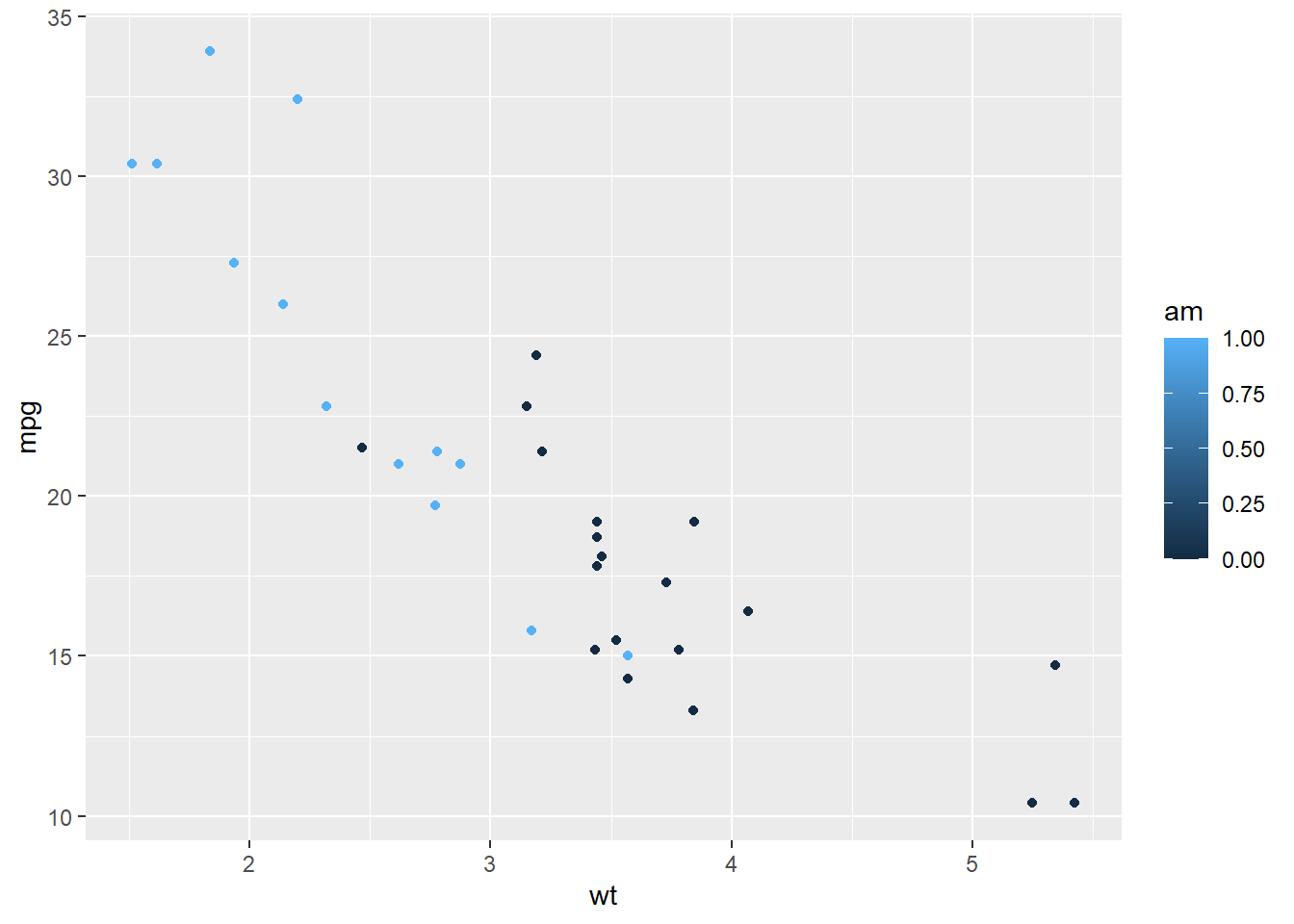
Add random noise to a variable
mtcarscopy <- mtcars

mtcarscopy$am <- mtcarscopy$am+runif(nrow(mtcarscopy),-1,1)
The jitter() function can also be useful for this:
mtcarscopy$am <- jitter(mtcarscopy$am)
Sum all variables into new a variable
Create a new variable called VarSum within dataset d which is the sum of all other variables in d:
The computer will add together the values for each variable in each row.
Sum all values of a variable
For entire dataset:
For a single variable:
colSums(as.data.frame(mtcars$cyl))[[1]]
Above, colSums can be changed to rowSums to sum up rows instead of columns.
Join words together
Use the paste(...) function:
something <- "three"
somethingelse <- "word"
anotherthing <- "phrase"
allthethingswithspaces <- paste(something, somethingelse, anotherthing)

allthethingswithspaces
## [1] "three word phrase"
allthethingswithoutspaces <- paste(something, somethingelse, anotherthing, sep = '')

allthethingswithoutspaces
## [1] "threewordphrase"
More or fewer than three items, separated by commas, can be added to the list of items in the paste(...) function. For example:
evenmorethings <- paste(something, somethingelse, anotherthing, anotherthing,something,somethingelse,somethingelse, sep = '')

evenmorethings
## [1] "threewordphrasephrasethreewordword"
Separate/split a variable into multiple dummy variables
d <- data.frame(person = c("Audi","Broof","Chruuma","Deenolo", "Eeman"),gender=c("A","A","B","B","B"), IceCreamFlavorsYouLikeSelectAllApply = c("chocolate","strawberry", "chocolate,vanilla","strawberry,vanilla,chocolate","vanilla,other") )

d
##    person gender IceCreamFlavorsYouLikeSelectAllApply
## 1    Audi      A                            chocolate
## 2   Broof      A                           strawberry
## 3 Chruuma      B                    chocolate,vanilla
## 4 Deenolo      B         strawberry,vanilla,chocolate
## 5   Eeman      B                        vanilla,other
Result not shown:
# Split the values in the column by commas
flavors <- strsplit(d$IceCreamFlavorsYouLikeSelectAllApply, ",")

# Get all unique ice cream flavors
unique_flavors <- unique(unlist(flavors))

# Create dummy variables for each unique flavor
for (flavor in unique_flavors) {
  # Create a new column with the flavor name and initialize with 0
  d[[flavor]] <- 0

  # Set the value to 1 if the flavor is in the list for that row
  d[[flavor]] <- as.integer(sapply(flavors, function(x) flavor %in% x))
}

d
The code above to create dummy variables was written by OpenAI’s GPT-3 model and accessed on 24 Sep 2023. This prompt was used: in r, i have a dataframe called d. there is a variable called IceCreamFlavorsYouLikeSelectAllApply in which each person (row in in the dataframe) might have one or multiple answers. some might say just ‘chocolate’ or ‘vanilla’ but others might say ’chocolate,vanilla,strawberry,other” or just “chocolate,strawberry”, for example. I want to create separate dummy variables in dataframe d for each of the ice cream flavors.
We get the code below with the following follow-up prompt to GPT-3: rewrite the code above so that each new variable will be called flavor_chocolate instead of just chocolate.
# Split the values in the column by commas
flavors <- strsplit(d$IceCreamFlavorsYouLikeSelectAllApply, ",")

# Get all unique ice cream flavors
unique_flavors <- unique(unlist(flavors))

# Create dummy variables with names like 'flavor_chocolate', 'flavor_vanilla', etc.
for (flavor in unique_flavors) {
  # Create a new column with the flavor name and initialize with 0
  d[[paste0("flavor_", flavor)]] <- 0

  # Set the value to 1 if the flavor is in the list for that row
  d[[paste0("flavor_", flavor)]] <- as.integer(sapply(flavors, function(x) flavor %in% x))
}

d
##    person gender IceCreamFlavorsYouLikeSelectAllApply flavor_chocolate
## 1    Audi      A                            chocolate                1
## 2   Broof      A                           strawberry                0
## 3 Chruuma      B                    chocolate,vanilla                1
## 4 Deenolo      B         strawberry,vanilla,chocolate                1
## 5   Eeman      B                        vanilla,other                0
##   flavor_strawberry flavor_vanilla flavor_other
## 1                 0              0            0
## 2                 1              0            0
## 3                 0              1            0
## 4                 1              1            0
## 5                 0              1            1
Follow-up prompt: how do i calculate summary counts and percentages of how many people like each flavor?
# Calculate summary counts for each flavor
flavor_counts <- colSums(d[paste0("flavor_", unique_flavors)])

# Calculate total number of respondents
total_respondents <- nrow(d)

# Calculate percentages
flavor_percentages <- (flavor_counts / total_respondents) * 100

# Create a summary dataframe
summary_df <- data.frame(Flavor = unique_flavors, Counts = flavor_counts, Percentages = flavor_percentages)

# Print the summary dataframe
print(summary_df)
##                       Flavor Counts Percentages
## flavor_chocolate   chocolate      3          60
## flavor_strawberry strawberry      2          40
## flavor_vanilla       vanilla      3          60
## flavor_other           other      1          20
Follow-up prompt (after a few attempts): we now have a dataframe called d with variables for gender as well as flavor_chocolate dummy variables and similar variables for each flavor. for each flavor, we need to know the count and what percentage of people in each gender group is equal to 1
# Load the dplyr package if not already loaded
# install.packages("dplyr")
library(dplyr)
##
## Attaching package: 'dplyr'
## The following objects are masked from 'package:stats':
##
##     filter, lag
## The following objects are masked from 'package:base':
##
##     intersect, setdiff, setequal, union
# Assuming you have a 'gender' column in your dataframe 'd'
# Calculate the count and percentage of each flavor for each gender
summary_df <- d %>%
  group_by(gender) %>%
  summarize(across(starts_with("flavor_"), ~sum(. == 1), .names = "Count_{.col}")) %>%
  mutate(across(starts_with("Count_"), ~. / sum(.), .names = "Percentage_{.col}"))

# Rename columns
colnames(summary_df) <- c("Gender", paste0("Count_", unique_flavors), paste0("Percentage_", unique_flavors))

# Print the summary data
print(summary_df)
## # A tibble: 2 × 9
##   Gender Count_chocolate Count_strawberry Count_vanilla Count_other
##   <chr>            <int>            <int>         <int>       <int>
## 1 A                    1                1             0           0
## 2 B                    2                1             3           1
## # ℹ 4 more variables: Percentage_chocolate <dbl>, Percentage_strawberry <dbl>,
## #   Percentage_vanilla <dbl>, Percentage_other <dbl>
Now we can transpose the result to make it easier to read (we also have to change gender into the column names):
summary_df <- t(summary_df)

colnames(summary_df) <- unlist(summary_df[1, ])
summary_df <- summary_df[-1, ]  # Remove the first row (which is now the column names)
And here’s a version that’s possibly simpler, for flavor counts by gender (result not shown):
d %>%
  group_by(gender) %>%
  summarise(
    count = n(),
    `count chocolate` = sum(flavor_chocolate, na.rm = TRUE),
    `count strawberry` = sum(flavor_strawberry, na.rm = TRUE)
  )
Output plain text
something <- "three"
somethingelse <- "word"
anotherthing <- "phrase"
cat(something, somethingelse, sep = '')
## threeword
allthethingswithspaces <- paste(something, somethingelse, anotherthing)

cat(allthethingswithspaces)
## three word phrase
Select rows (observations) from a dataset
Select first 50 rows:
Select individual rows (in this example, select rows 3, 17, 22):
d.new <- d.old[c(3,17,22),]
Select rows (observations) from a dataset using dplyr filter
library(dplyr)
mtcars %>% filter(cyl==4)
Save a copy:
mtcars.cyl4 <- mtcars %>% filter(cyl==4)
Remove rows (observations) from a dataset, based on negative criteria
Create a new data set called newdata.cars that contains the observations (rows) in mtcars that do NOT have cyl equal to 8.
newdata.cars <- mtcars[ which(mtcars$cyl!=8), ]

table(mtcars$cyl)
table(newdata.cars$cyl)
Above, we see that the 14 cars with 8 cylinders were removed from the original data.
Remove rows (observations) from a dataset, based on observation numbers
Remove first 50 rows:
d.new <- d.old[-c(1:50),]
Remove selected rows (in this example, remove rows 3, 17, 22):
d.new <- d.old[-c(3,17,22),]
Remove all rows except header (to create an empty dataset while preserving column names):
d.new <- d.old[-c(1:nrow(d.old)),]
Subset based on multiple qualitative variable levels
d <- data.frame(name = c("Aabe","Bobay","Chock","Deela","Edweeeena","Foort","Gooba","Hi"),
                group = c("A","A","B","B","C","C","D","D")
                )

dpartial <- d[d$group %in% c("A", "B"), ]
Subset and rename selected variables (columns)
library(dplyr)
newData <- mtcars %>% dplyr::select(mileage=mpg, transmission=am)
Rename selected variables (columns)
library(dplyr)
newData <- mtcars %>% dplyr::rename(mileage=mpg, transmission=am)
Remove selected variables (columns) from a dataset
Remove variable Var1 from dataset d:
d$Var1 <- NULL
Remove variable mpg from the data set mtcars and save the new version of the data set as d:
d <- subset(mtcars, select = -mpg)
Remove variables mpg, cyl, and carb from the data set mtcars and save it as d:
d <- subset(mtcars, select = -c(mpg, cyl, carb))
Above, deleting the - sign in the select argument will keep (rather than remove) the listed variables and remove all others.
Using dplyr, remove variable Var1 from dataset d:
library(dplyr)
d <- d %>% select(-Var1)
Using dplyr, remove variables Var1 and Var2 from dataset d:
library(dplyr)
d <- d %>% select(-Var1,-Var2)
Remove variables with missing data
Option 1
This removes all variables that have one or more missing values:
NewData <- OldData[ , colSums(is.na(OldData)) == 0]
The code above was taken from the following resource:
Option 2
Remove all variables which contain only NA values:
NewData <- OldData[ , colSums(is.na(OldData)) < nrow(OldData)]
The code above was taken from the following resource:
Remove non-numeric variables from a dataset
Example data:
d <- data.frame(
  name = factor(c("Aronda","Baeoi","Chromp","Daroona")),
  age = c(23,45,56,67),
  citizenship = c("Tanzania","Nigeria","Mexico","France"),
  educationYears = c(1,2,3,4)
)

d
##      name age citizenship educationYears
## 1  Aronda  23    Tanzania              1
## 2   Baeoi  45     Nigeria              2
## 3  Chromp  56      Mexico              3
## 4 Daroona  67      France              4
## 'data.frame':    4 obs. of  4 variables:
##  $ name          : Factor w/ 4 levels "Aronda","Baeoi",..: 1 2 3 4
##  $ age           : num  23 45 56 67
##  $ citizenship   : chr  "Tanzania" "Nigeria" "Mexico" "France"
##  $ educationYears: num  1 2 3 4
Remove non-numeric variables:
dNumericOnly <- d[,sapply(d, is.numeric)]
View new data:
##   age educationYears
## 1  23              1
## 2  45              2
## 3  56              3
## 4  67              4
Do something with the data that you couldn’t do before:
##                      age educationYears
## age            1.0000000      0.9827076
## educationYears 0.9827076      1.0000000
keywords: keep numeric variables, retain numeric variables
Identical variables in two datasets
Let’s say you have one dataset called dtrain and another one called dtest. And you want to make sure that dtest has the same variables (columns) as dtrain.
The code below tells the computer to retain within dtest only the variables that are in dtrain:
library(dplyr)
dtest <- dtest %>% select(names(dtrain))
Remove observations with missing values (NA values) in a single column
Take the existing dataframe OldData and make a new dataframe called NewData which only contains the rows in OldData that do NOT have a missing value—meaning do not have NA—for a variable called Var1:
NewData <- OldData[which(!is.na(OldData$Var1)),]
NewData should be a version of OldData in which any observation (row) coded as NA for Var1 has been removed.
Replace missing values (NA values) with 0
In an entire dataset
my_dataframe[is.na(my_dataframe)] <- 0
In one column of the dataset
my_dataframe["pages"][is.na(my_dataframe["pages"])] <- 0
Combine or concatenate strings
s <- ""
s1 <- "something"
s2 <- "Else"
s <- paste(s, s1, s2, sep = "")

s
## [1] "somethingElse"
Search vector or variable for values
x <- c(1,2,3,4,5)
any(x>5)
## [1] FALSE
## [1] TRUE
Search to see if a row is contained in a data frame
Let’s say we want to check if mtcars contains any rows with am = 1, gear = 5, and carb = 6:
## ------------------------------------------------------------------------------
## You have loaded plyr after dplyr - this is likely to cause problems.
## If you need functions from both plyr and dplyr, please load plyr first, then dplyr:
## library(plyr); library(dplyr)
## ------------------------------------------------------------------------------
##
## Attaching package: 'plyr'
## The following objects are masked from 'package:dplyr':
##
##     arrange, count, desc, failwith, id, mutate, rename, summarise,
##     summarize
match_df(mtcars, data.frame(am=1, gear=5, carb=6))
## Matching on: am, gear, carb
##               mpg cyl disp  hp drat   wt qsec vs am gear carb
## Ferrari Dino 19.7   6  145 175 3.62 2.77 15.5  0  1    5    6
And now let’s test for something that doesn’t exist:
library(plyr)
match_df(mtcars, data.frame(am=1, gear=5, carb="bobb"))
## Matching on: am, gear, carb
##  [1] mpg  cyl  disp hp   drat wt   qsec vs   am   gear carb
## <0 rows> (or 0-length row.names)
Search for text strings in variables
Given a dataset like d below, identify which names do and do not contain any of the strings ee and a:
d <- data.frame(Name = c("Aweo","Beena","Cidu","Deleek","Erga", "Fymo","Henny"), LevelOfInterest = c(3,1,2,3,2,1,2))
searchStrings <- c("ee","a")

d$searchMatch <- grepl(paste(toupper(searchStrings),collapse="|"), toupper(d$Name))

d
##     Name LevelOfInterest searchMatch
## 1   Aweo               3        TRUE
## 2  Beena               1        TRUE
## 3   Cidu               2       FALSE
## 4 Deleek               3        TRUE
## 5   Erga               2        TRUE
## 6   Fymo               1       FALSE
## 7  Henny               2       FALSE
In each row in d, searchMatch is TRUE if Name contains at least one of the strings in searchStrings.
Look up or search for a single item or value
## [1] 32.4
Randomly reorder/resort data set
One-line version
Quick code to randomly reorder df and save it still as df:
df <- df[sample(1:nrow(df)), ]
More details
Re-sort myOriginalData and save it as myRandomlySortedData:
myOriginalData <- mtcars

rows <- sample(nrow(myOriginalData))
myRandomlySortedData <- myOriginalData[rows, ]
Check if it worked (results not shown):
head(myOriginalData)
head(myRandomlySortedData)
Quick code to randomly order df and save it still as df:
df <- df[sample(1:nrow(df)), ]
Sort/order data set by one or more variables
Sort dataframe oldData by Var1 from low to high:
newData <- oldData[order(oldData$Var1),]
Sort dataframe oldData by Var1 from high to low:
newData <- oldData[order(-oldData$Var1),]
Sort dataframe oldData by Var1 and then Var2, both from low to high:
newData <- oldData[order(oldData$Var1, oldData$Var2),]
Sort dataframe oldData by Var1 from low to high and then Var2 from high to low:
newData <- oldData[order(oldData$Var1, -oldData$Var2),]
- The code above has not been tested for accuracy, as of July 22 2021.
Create a rank variable based on another variable
In the dataset below, we want to take each student’s score and use that to determine their rank in the class.
(d <- data.frame(studentName = c("Aabe","Beebe","Cheech","Doola","Eena","Fon"), score = c(77,89,45,33,99,77)))
##   studentName score
## 1        Aabe    77
## 2       Beebe    89
## 3      Cheech    45
## 4       Doola    33
## 5        Eena    99
## 6         Fon    77
d$classRank <- rank(d$score)

d
##   studentName score classRank
## 1        Aabe    77       3.5
## 2       Beebe    89       5.0
## 3      Cheech    45       2.0
## 4       Doola    33       1.0
## 5        Eena    99       6.0
## 6         Fon    77       3.5
Above, we now have a classRank variable which identifies how each student compares to the rest on score.
Count the occurrence number of each subject or within each group
Below, we have a data frame d1:
d1 <- data.frame(subjectID = c("a","a","a","b","b"))

d1
##   subjectID
## 1         a
## 2         a
## 3         a
## 4         b
## 5         b
We want a new variable that counts how many times each subject appears in the data:
library(dplyr)

d2 <- d1 %>%
      dplyr::group_by(subjectID) %>%
      dplyr::mutate(withinPersonRecordNumber = row_number()) %>%
      ungroup()

d2
## # A tibble: 5 × 2
##   subjectID withinPersonRecordNumber
##   <chr>                        <int>
## 1 a                                1
## 2 a                                2
## 3 a                                3
## 4 b                                1
## 5 b                                2
If needed, we can only keep the first row for each subject:
d3 <- d2 %>% filter(withinPersonRecordNumber==1)

d3
## # A tibble: 2 × 2
##   subjectID withinPersonRecordNumber
##   <chr>                        <int>
## 1 a                                1
## 2 b                                1
Count the frequency (number of times) that a single subject ID or variable value/level occurs
Below, we have a data frame d1:
d1 <- data.frame(subjectID = c("a","a","a","b","b"))

d1
##   subjectID
## 1         a
## 2         a
## 3         a
## 4         b
## 5         b
We want a new variable that counts how often each subject appears in the data:
library(dplyr)

d2 <- d1 %>%
  add_count(subjectID, name = "Frequency")

d2
##   subjectID Frequency
## 1         a         3
## 2         a         3
## 3         a         3
## 4         b         2
## 5         b         2
Change variable names to numbers
d <- mtcars
colnames(d) <- seq(1:ncol(d))
Select start of variable name
Select variables that start with the characters StartOfVar1 and apple
library(dplyr)
NewData <- OldData %>% select(someVariableIwant,starts_with(c("StartOfVar1","apple")))
NewData will now contain the variable someVariableIwant from OldData as well as any in OldData that start with the characters StartOfVar1 or apple.
If you don’t want someVariableIwant to be included, you can just do this:
NewData <- OldData %>% select(starts_with(c("StartOfVar1","apple")))
Select numeric variables
Create a copy of olddata which only contains numeric variables and we save it as newdata:
library(dplyr)
newdata <- olddata %>% select_if(is.numeric)
Select variables from another data set
mtcars.temp <- mtcars[c("mpg","cyl")]

mtcars.copy1 <- mtcars[names(mtcars.temp)]
Above, mtcars.copy1 contains the same variables that are in mtcars.temp, taken from mtcars.
Converting categorical and numeric data
The following code converts a numeric variable to a categorical one:
DataSet$NewVariable <- as.factor(DataSet$OldVariable)
The following code converts a factor (categorical) variable to a numeric one:
DataSet$NewVariable <- as.numeric(as.character(DataSet$OldVariable))
Check what type of data is in each variable:
DataSet$OldVariable
DataSet$NewVariable
Here is how we can convert a numeric variable to a categorical variable and then relabel the values:
mtcarscopy <- mtcars
mtcarscopy$amfactor <- as.factor(mtcarscopy$am)

library(plyr)
plyr::revalue
## function (x, replace = NULL, warn_missing = TRUE)
## {
##     if (!is.null(x) && !is.factor(x) && !is.character(x)) {
##         stop("x is not a factor or a character vector.")
##     }
##     mapvalues(x, from = names(replace), to = replace, warn_missing = warn_missing)
## }
## <bytecode: 0x00000286eb1525d8>
## <environment: namespace:plyr>
mtcarscopy$amlabeled <- revalue(mtcarscopy$amfactor, c("0"="automatic", "1"="manual"))

head(mtcarscopy[c("am", "amfactor", "amlabeled")], n=10)
##                   am amfactor amlabeled
## Mazda RX4          1        1    manual
## Mazda RX4 Wag      1        1    manual
## Datsun 710         1        1    manual
## Hornet 4 Drive     0        0 automatic
## Hornet Sportabout  0        0 automatic
## Valiant            0        0 automatic
## Duster 360         0        0 automatic
## Merc 240D          0        0 automatic
## Merc 230           0        0 automatic
## Merc 280           0        0 automatic
Converting likert responses to numeric and summing up totals
Initial data, called d.original:
d.original <- data.frame(
  name = c("Abby","Beeta","Chock"),
  Q1 = c("2 - somewhat bad","3 - neutral","5 - very good"),
  Q2 = c("4 - somewhat good","1 - very bad","3 - neutral"),
  Q3 = c("2 - somewhat bad","5 - very good","2 - somewhat bad")
                )
Make likertFix function to handle data like this:
likertFix <- function(df, questionPrefix="", variablePrefix=""){

  # df is the dataset you're starting with
  # questionPrefix is the characters in quotation marks that label relevant columns for conversion to numbers and totaling up
  # variablePrefix is a short word in quotation marks that you want to label the columns being fixed and added

  df.q <- df %>% select(starts_with(questionPrefix))
  df.q[] <- lapply(df.q, function(x) substring(x,1,1))
  df.q[] <- lapply(df.q, function(x) as.numeric(x))
  df.q$total <- rowSums(df.q)
  colnames(df.q) <- paste(variablePrefix, colnames(df.q), sep = ".")
  df <- cbind(df,df.q)
  df <- df %>% select(-starts_with(questionPrefix))
  return(df)
}
Run the likertFix function on the initial data and save the result
dfixed <- likertFix(df = d.original, questionPrefix = "Q", variablePrefix = "Pretest")
dfixed
##    name Pretest.Q1 Pretest.Q2 Pretest.Q3 Pretest.total
## 1  Abby          2          4          2             8
## 2 Beeta          3          1          5             9
## 3 Chock          5          3          2            10
Assign reference group or reference category in factor variables
Generic code:
mydata$variableToFix <- relevel(as.factor(mydata$variableToFix), ref = "Label of reference group")
Example in which we want to use the cyl variable in mtcars (which we’ll re-save as d) as a factor variable with 6 as the reference group:
d<-mtcars
d$newCyl <- relevel(as.factor(d$cyl), ref = "6")

summary(lm(mpg~newCyl,d))
##
## Call:
## lm(formula = mpg ~ newCyl, data = d)
##
## Residuals:
##     Min      1Q  Median      3Q     Max
## -5.2636 -1.8357  0.0286  1.3893  7.2364
##
## Coefficients:
##             Estimate Std. Error t value Pr(>|t|)
## (Intercept)   19.743      1.218  16.206 4.49e-16 ***
## newCyl4        6.921      1.558   4.441 0.000119 ***
## newCyl8       -4.643      1.492  -3.112 0.004152 **
## ---
## Signif. codes:  0 '***' 0.001 '**' 0.01 '*' 0.05 '.' 0.1 ' ' 1
##
## Residual standard error: 3.223 on 29 degrees of freedom
## Multiple R-squared:  0.7325, Adjusted R-squared:  0.714
## F-statistic:  39.7 on 2 and 29 DF,  p-value: 4.979e-09
As we can see above, cars with 6 cylinders were omitted because they’re in the reference group.
Assign values in dataframe based on matched criteria
Below, set mpg equal to 200 for all observations for which am = 0, gear = 0, and carb = 2.
d <- mtcars

d[which(d$am==0 & d$gear==3 & d$carb==2),]$mpg <- 200

mtcars
Save table as dataframe
tableAMxCYL <- with(mtcars, table(am, cyl, useNA = 'ifany'))
dfAMxCYL <- as.data.frame.matrix(tableAMxCYL)
dfAMxCYL
Add am column as variable:
dfAMxCYL$am <- rownames(dfAMxCYL)
dfAMxCYL
Convert all columns in data frame to numeric
dNew <- sapply(dOriginal, as.numeric)
Read more:
Make a copy of an object
Make a copy of df called dfcopy:
This can be done for any object like a dataset, stored value, regression object, and so on.
Remove missing data
Remove rows in dataset df that contain any missing data:
df <- na.omit(df)
Reverse code a numeric variable
If you have a variable like LevelOfInterest in the dataset d below…
d <- data.frame(Name = c("Aweo","Been","Cida","Deleek","Erga"), LevelOfInterest = c(3,1,2,3,2))

d
##     Name LevelOfInterest
## 1   Aweo               3
## 2   Been               1
## 3   Cida               2
## 4 Deleek               3
## 5   Erga               2
…you might want to change it so that:
- 3 becomes 1
- 2 remains 2
- 1 becomes 3
This might help you do that:
d$LevelOfInterest.reverse <- (max(d$LevelOfInterest, na.rm = T)+1)-d$LevelOfInterest
Use a two-way table to see if this worked:
with(d, table(LevelOfInterest, LevelOfInterest.reverse))
##                LevelOfInterest.reverse
## LevelOfInterest 1 2 3
##               1 0 0 1
##               2 0 2 0
##               3 2 0 0
This code should work even for a variable with greater or less than three levels.
This issue is discussed more here:
Put row names into a variable
d <- mtcars # example data

d$carName <- rownames(d) # make a new variable called carName containing the row names of d

View(d) # check if it worked
Assign row names based on a variable
# example data
d <- data.frame(name = c("Kazaan","Kaalaa","Koona"), age = c(1,2,3), employed = c("no","no","no"))

rownames(d) <- d$name # change row names to be the wt of each car

View(d) # check if it worked
Check if values in one variable are in another variable
entireGroup <- data.frame(name = c("Beebo","Brakaansha","Bettle","Bo","Erl"), age = c(23,45,93,23,4))
signedUpList <- data.frame(writtenName = c("Bettle","Bo"), profession = c("Sword swallower swallower", "Anti snake charming activist"))

entireGroup$signedUp <- ifelse(entireGroup$name %in% signedUpList$writtenName, 1,0)

entireGroup
##         name age signedUp
## 1      Beebo  23        0
## 2 Brakaansha  45        0
## 3     Bettle  93        1
## 4         Bo  23        1
## 5        Erl   4        0
Unique identifiers
Make a unique identification (ID) number for observations or groups of observations.
Simple ID number by row
Add a new variable with the row number of each observation:
YourDataFrame$IDnum <- seq(1:nrow(YourDataFrame))
More complicated ID numbers
Sample data to practice with:
d <- data.frame(name = c("Aaaaaaron","Beela","Cononan","Duh","Eeena","Beela","Eeena","Beela"), age = c(1,2,3,4,1,2,1,2), occupation = c("hunter","vegan chef","plumber","plumbing destroyer","omnivore chef","vegan chef","omnivore chef","vegan chef"), day = c(1,1,1,1,15,15,15,15), month = c("January","February","March","April","January","February","March","April"), year = rep(2020,8), result = seq(1,8))

d
##        name age         occupation day    month year result
## 1 Aaaaaaron   1             hunter   1  January 2020      1
## 2     Beela   2         vegan chef   1 February 2020      2
## 3   Cononan   3            plumber   1    March 2020      3
## 4       Duh   4 plumbing destroyer   1    April 2020      4
## 5     Eeena   1      omnivore chef  15  January 2020      5
## 6     Beela   2         vegan chef  15 February 2020      6
## 7     Eeena   1      omnivore chef  15    March 2020      7
## 8     Beela   2         vegan chef  15    April 2020      8
Generate variable ID in dataset d containing a unique identification number for each person:
if (!require(udpipe)) install.packages('udpipe')
library(udpipe)

d$ID <- unique_identifier(d, c("name"))

d
##        name age         occupation day    month year result ID
## 1 Aaaaaaron   1             hunter   1  January 2020      1  1
## 2     Beela   2         vegan chef   1 February 2020      2  2
## 3   Cononan   3            plumber   1    March 2020      3  3
## 4       Duh   4 plumbing destroyer   1    April 2020      4  4
## 5     Eeena   1      omnivore chef  15  January 2020      5  5
## 6     Beela   2         vegan chef  15 February 2020      6  2
## 7     Eeena   1      omnivore chef  15    March 2020      7  5
## 8     Beela   2         vegan chef  15    April 2020      8  2
More sample data for practice:
d2 <- data.frame(name = c("Aaaaaaron","Beela","Cononan","Duh","Eeena","Fewe","Graam","Hiol"), number = c(1,1,1,1,0,0,0,0), color = c("green","brown","green","brown","green","brown","green","brown"))

d2
##        name number color
## 1 Aaaaaaron      1 green
## 2     Beela      1 brown
## 3   Cononan      1 green
## 4       Duh      1 brown
## 5     Eeena      0 green
## 6      Fewe      0 brown
## 7     Graam      0 green
## 8      Hiol      0 brown
Generate variable group in dataset d2 containing a unique identification number for each number-color pair:
if (!require(udpipe)) install.packages('udpipe')
library(udpipe)

d2$group <- unique_identifier(d2, c("number","color"))

d2
##        name number color group
## 1 Aaaaaaron      1 green     4
## 2     Beela      1 brown     3
## 3   Cononan      1 green     4
## 4       Duh      1 brown     3
## 5     Eeena      0 green     2
## 6      Fewe      0 brown     1
## 7     Graam      0 green     2
## 8      Hiol      0 brown     1
Within-group count of observations and group size, within-group ID number
If you have multiple observations in one group or for one person and you need to count each observation’s number within each group or person, the code below should help.
# Install and load the required package
library(dplyr)

# Create an example dataframe
df <- data.frame(
  person = c("John", "John", "Mary", "Mary", "Mary", "Peter"),
  age = c(25, 30, 35, 40, 45, 50)
)

# Create a new variable with the count of rows for each person
df <- df %>%
  dplyr::group_by(person) %>%
  dplyr::mutate(row_count = row_number()) %>%
  ungroup()

# Print the modified dataframe
print(df)
The code and comments above were generated by ChatGPT on May 22 2023, with minor modifications by Anshul.
If you want to generate a group size variable instead, this might help:
# Install and load the required package
library(dplyr)

# Create an example dataframe
df <- data.frame(
  person = c("John", "John", "Mary", "Mary", "Mary", "Peter"),
  age = c(25, 30, 35, 40, 45, 50)
)

# Create a new variable with the count of rows for each person
df <- df %>%
  dplyr::group_by(person) %>%
  dplyr::mutate(row_count = n()) %>%
  ungroup()

# Print the modified dataframe
print(df)
The code and comments above were generated by ChatGPT on May 22 2023.
Make new character variable or summary report based on other variables
Example data:
d <- data.frame(
  flavor = c("chocolate","vanilla","strawberry","other"),
  numberEaten = c(1,2,3,4)
)
d$joinedVariable <- paste0("Flavor and number: ",as.character(d$flavor)," ", as.character(d$numberEaten))
##       flavor numberEaten                  joinedVariable
## 1  chocolate           1  Flavor and number: chocolate 1
## 2    vanilla           2    Flavor and number: vanilla 2
## 3 strawberry           3 Flavor and number: strawberry 3
## 4      other           4      Flavor and number: other 4
Source: Solution by user sandeep. Concatenating two string variables in r. https://stackoverflow.com/questions/26321702/concatenating-two-string-variables-in-r.
keywords: concatenate, join
Converting time variables in R
You might have data in which there are time stamps which you need to convert into a continuous variable that you can put into a regression. For example, maybe you have data in which each row (observation) is a patient and then you have a variable (column) for the date and time on which the patient came into the hospital. To analyze this data as a continuous variable, maybe you want to calculate how many seconds after midnight in each day a patient came in.
How can we convert a time to a number of seconds? There are helper functions in R that help us do this. Let’s start with an example:
if (!require(lubridate)) install.packages('lubridate')
## Warning: package 'lubridate' was built under R version 4.2.3
library(lubridate) # this package has the period_to_seconds function

# example of what the data looks like
ExampleTimestamp <- "01-01-2019 09:04:58"

# extract just the time (remove the date)
(ExampleTimeOnly <- substr(ExampleTimestamp,12,19))
## [1] "09:04:58"
# convert from time to number of seconds
(TotalSeconds <- period_to_seconds(hms(ExampleTimeOnly)))
## [1] 32698
As you can see above, the time “09:04:59” was converted into 32698 seconds. But we only did it for a single stored value, ExampleTimestamp. How do we do it for the entire variable in a dataset? Let’s say you have a datset called d with a variable with a time stamp called timestamp and you want to make a new variable (column) in the dataset called seconds. Here’s how you can do it:
if (!require(lubridate)) install.packages('lubridate')
library(lubridate)

d$seconds <- period_to_seconds(hms(substr(d$timestamp,12,19)))
Making and modifying lists
This is not complete.
l <- list() # make empty list
l <- append(l, "bob") # add something to the list
one <- 1
two <- c(1,2,3,4)
three <- list("byron","anshul")
four <- "bob"
t <- list(one, two, three) # make a list

t <- append(t, four) # add something to the list
Categorize variable into quantiles
Make a new variable called quintile that identifies each observation’s quintile for the variable mpg:
d <- mtcars
d$mpg[4] <- NA # create missing data for illustration only

library(dplyr)
d$mpg.quintile <- ntile(d$mpg, 5)
Check if it worked:
table(d$mpg.quintile, useNA = "always")
class(d$mpg.quintile)
As an option, recode the new variable as a factor and label NA values as missing, so that the computer doesn’t know they are NA anymore (the NA observations won’t get thrown out of an analysis):
d$mpg.quintile.fac <- ifelse(is.na(d$mpg.quintile), "missing",as.character(d$mpg.quintile))
table(d$mpg.quintile.fac, useNA = "always")
class(d$mpg.quintile.fac)
Combine similar levels into groups
This is incomplete. See this reference:
Merging and joining datasets together
left <- data.frame(name=c("A. Onlyleft","B. Onlyleft","C. Both","D. Both", NA), skill=c("pig latin","latin","pig farming","pig surgery","pig liberating"))
left
##          name          skill
## 1 A. Onlyleft      pig latin
## 2 B. Onlyleft          latin
## 3     C. Both    pig farming
## 4     D. Both    pig surgery
## 5        <NA> pig liberating
right <- data.frame(name = c("E. Onlyright","F. Onlyright","C. Both","D. Both", NA), skill=c("reading","writing","speling","boating","gloating"))
right
##           name    skill
## 1 E. Onlyright  reading
## 2 F. Onlyright  writing
## 3      C. Both  speling
## 4      D. Both  boating
## 5         <NA> gloating
leftjoined <- dplyr::left_join(left, right, by="name")
leftjoined
##          name        skill.x  skill.y
## 1 A. Onlyleft      pig latin     <NA>
## 2 B. Onlyleft          latin     <NA>
## 3     C. Both    pig farming  speling
## 4     D. Both    pig surgery  boating
## 5        <NA> pig liberating gloating
rightjoined <- dplyr::right_join(left, right, by="name")
rightjoined
##           name        skill.x  skill.y
## 1      C. Both    pig farming  speling
## 2      D. Both    pig surgery  boating
## 3         <NA> pig liberating gloating
## 4 E. Onlyright           <NA>  reading
## 5 F. Onlyright           <NA>  writing
fulljoined <- dplyr::full_join(left, right, by="name")
fulljoined
##           name        skill.x  skill.y
## 1  A. Onlyleft      pig latin     <NA>
## 2  B. Onlyleft          latin     <NA>
## 3      C. Both    pig farming  speling
## 4      D. Both    pig surgery  boating
## 5         <NA> pig liberating gloating
## 6 E. Onlyright           <NA>  reading
## 7 F. Onlyright           <NA>  writing
merged <- merge(left, right, by="name", all = TRUE, incomparables = NA)
# all.x or all.y also possible to do only left or right joins
# change to all=F to only include observations that match
merged
##           name        skill.x  skill.y
## 1  A. Onlyleft      pig latin     <NA>
## 2  B. Onlyleft          latin     <NA>
## 3      C. Both    pig farming  speling
## 4      D. Both    pig surgery  boating
## 5 E. Onlyright           <NA>  reading
## 6 F. Onlyright           <NA>  writing
## 7         <NA> pig liberating     <NA>
## 8         <NA>           <NA> gloating
What if we wanted to make a new variable called dataSource which identifies who all came from which dataset? I’m not sure of the very best way to do it, but here’s one way that seems to work:
left$inLeft <- 1
right$inRight <- 1

merged2 <- merge(left, right, by="name", all = TRUE, incomparables = NA)

merged2$dataSource <- NA
merged2$dataSource[merged2$inLeft==1 & merged2$inRight==1] <- "Present in both left and right"
merged2$dataSource[merged2$inLeft==1 & is.na(merged2$inRight)] <- "Present in left only"
merged2$dataSource[is.na(merged2$inLeft) & merged2$inRight==1] <- "Present in right only"

merged2
##           name        skill.x inLeft  skill.y inRight
## 1  A. Onlyleft      pig latin      1     <NA>      NA
## 2  B. Onlyleft          latin      1     <NA>      NA
## 3      C. Both    pig farming      1  speling       1
## 4      D. Both    pig surgery      1  boating       1
## 5 E. Onlyright           <NA>     NA  reading       1
## 6 F. Onlyright           <NA>     NA  writing       1
## 7         <NA> pig liberating      1     <NA>      NA
## 8         <NA>           <NA>     NA gloating       1
##                       dataSource
## 1           Present in left only
## 2           Present in left only
## 3 Present in both left and right
## 4 Present in both left and right
## 5          Present in right only
## 6          Present in right only
## 7           Present in left only
## 8          Present in right only
General R use and processes
Run R in web browser without signing in
This should work on your phone, too!
Check R version and packages
See which version of R you are using, which packages are loaded, and other information about the current session of R:
Remove an object from the environment
Remove df from the environment in R:
Remove all objects from the environment
Get code to recreate a dataframe or object
Fix variable names automatically
With a data set called d:
names(d) <- make.names(names(d))
See the changes:
More information:
List all variables in a dataset
The following code outputs a list of all variables in the dataset mtcars, in quotation marks and separated by commas:
for(n in names(mtcars)){cat('"',n,'",', sep='')}
## "mpg","cyl","disp","hp","drat","wt","qsec","vs","am","gear","carb",
- In the code above, replace
mtcars with the name of your own dataset.
- There will be an extra—likely unwanted—comma at the end of the list.
This code can give you a list of your variables to manually modify and then paste into a regression formula:
for(n in names(mtcars)){cat(' + ',n, sep='')}
## + mpg + cyl + disp + hp + drat + wt + qsec + vs + am + gear + carb
This does the same thing:
(VarListString <- paste(names(mtcars), collapse="+"))
## [1] "mpg+cyl+disp+hp+drat+wt+qsec+vs+am+gear+carb"
Without quotation marks:
cat(paste(names(mtcars), collapse="+"))
## mpg+cyl+disp+hp+drat+wt+qsec+vs+am+gear+carb
List all objects in R environment
##  [1] "age"                          "allthethingswithoutspaces"
##  [3] "allthethingswithspaces"       "anotherthing"
##  [5] "bw"                           "c1"
##  [7] "c2"                           "cc"
##  [9] "d"                            "d.original"
## [11] "d1"                           "d2"
## [13] "d3"                           "demographics"
## [15] "descriptivetable"             "descriptivetable.abbreviated"
## [17] "descriptivetable.transpose"   "df"
## [19] "dfcopy"                       "dfixed"
## [21] "dNumericOnly"                 "dpartial"
## [23] "Engine"                       "entireGroup"
## [25] "eqn"                          "evenmorethings"
## [27] "ExampleTimeOnly"              "ExampleTimestamp"
## [29] "first"                        "flavor"
## [31] "flavor_counts"                "flavor_percentages"
## [33] "flavors"                      "four"
## [35] "fulljoined"                   "GroupMeanData"
## [37] "hgA"                          "hgB"
## [39] "l"                            "left"
## [41] "leftjoined"                   "likertFix"
## [43] "med_df"                       "merged"
## [45] "merged2"                      "mtcars.copy1"
## [47] "mtcars.partial"               "mtcars.temp"
## [49] "mtcarscopy"                   "n"
## [51] "name"                         "one"
## [53] "pca1"                         "post"
## [55] "pre"                          "reg"
## [57] "right"                        "rightjoined"
## [59] "s"                            "s1"
## [61] "s2"                           "searchStrings"
## [63] "second"                       "signedUpList"
## [65] "something"                    "somethingelse"
## [67] "summary_df"                   "t"
## [69] "test"                         "three"
## [71] "total_respondents"            "TotalSeconds"
## [73] "Transmission"                 "two"
## [75] "unique_flavors"               "VarListString"
## [77] "x"                            "zipcodes"
If you see character(0) as the output, that means the environment is empty.
List all files in current working directory or a selected directory
Working directory:
A selected directory:
list.files("C:/Users/MyUserName/Path/To/Desired/Folder")
Assigning new values or making copies
Here’s how you make a copy of anything in R:
The code above is doing the following:
- Create a new object called
thing1
- The
<- operator assigns whatever is on the right to whatever is on the left.
- Assign
thing1 to be the value of thing2. thing2 still exists too, note.
You can also make a copy of a dataset like this:
library(car)
d <- GSSvocab
This makes a copy of the dataset GSSvocab called d. Then you can just use this dataset without having to type GSSvocab each time.
Run code from one R file in another R file
It is possible to run load functions and run code from other files in one file.
If…
- Your first file is called
one.R
- Your second file is called
two.R
Then you can run the command
source('one.R')
within the file called two.R and all of the code in the file one.R will be run as if it was run from within the file two.R.
Make sure that the file one.R is in your working directory.
More information:
Count how long a process in R takes
To measure or count the duration of how long it takes for R to run something for you, you can put the code
(start <- Sys.time())
and
(end <- Sys.time())
(duration <- end-start)
around the code you want to measure/count.
Let’s say you want to load a data file into R using the code d <- read.csv("SomeData.csv") and you want to measure how long it takes to load the file. You would write this code:
(start <- Sys.time())
d <- read.csv("SomeData.csv")
(end <- Sys.time())
(duration <- end-start)
Above, the stored object duration contains the amount of time it took to load the data file.
Save R objects to a folder on the computer
Let’s say you have an R object called MyRobject, which could be a dataframe, saved regression model, table, or anything else.
You can save that R object to your computer like this (it will go to the working directory or directory where your code file is):
saveRDS(MyRobject, file = "ChooseAname.rds")
With the code above, MyRobject will be saved as a file on your computer with the name ChooseAname.rds. You can of course change it to a name other than ChooseAname.rds.
Later, when you want to open the saved object again in RStudio, you can run this code:
MyRobjectFromBefore <- readRDS("ChooseAname.rds")
Above, we load the object saved in ChooseAname.rds into R, where it will have the name MyRobjectFromBefore. Of course you can choose to call it anything other than MyRobjectFromBefore.
Here is the code above once again, for easy copying and pasting:
saveRDS(obj, file = "obj.rds")
obj <- readRDS("obj.rds")
Get the name of an object or dataframe as a string
Below, the name of the dataset mtcars will be printed out as a string:
deparse(substitute(mtcars))
## [1] "mtcars"
We could also save the string:
theSavedString <- deparse(substitute(mtcars))

theSavedString
## [1] "mtcars"
Get the R code for a saved object
Let’s say we have a stored object and we want the R code that was used to create it, we can use dput():
## c(21, 21, 22.8, 21.4, 18.7, 18.1, 14.3, 24.4, 22.8, 19.2, 17.8,
## 16.4, 17.3, 15.2, 10.4, 10.4, 14.7, 32.4, 30.4, 33.9, 21.5, 15.5,
## 15.2, 13.3, 19.2, 27.3, 26, 30.4, 15.8, 19.7, 15, 21.4)
Generating R code using R
Parsing and running code from saved strings
Below, the eval(...) function treats a string as if it is R code, and tries to run it.
target <- "myvector"
values <- "c(1,2,3,4)"

eval(parse(text=paste(target, " <- ", values, sep = "")))
myvector
## [1] 1 2 3 4
The code above made the computer run the following:
target and values are saved strings of characters.- Replace
target, " <- ", values with anything you want and R will run it as if it is R code.
- More than just
target, <-, and values can be added to the comma separated list within the paste(...) function. The list can be endless.
Check if one string is contained in another string
##
## Attaching package: 'stringr'
## The following objects are masked from 'package:expss':
##
##     fixed, regex
str_detect("this is the text that the computer will search within","this is the string the computer is trying to find within the other text")
## [1] FALSE
Replace/substitute text in strings
gsub("replacement text", "text to be replaced", "string of text in which there is some text to be replaced")
new <- "blue"
old <- "red"
oldtext <- "On Mondays, my favorite color is red"

newtext <- gsub(new, old, oldtext)

newtext
Read more (including a more complex and useful example):
Using packages
Install and load a package
if (!require(packagename)) install.packages('packagename')
library(packagename)
- Replace
packagename with the name of the package you want to use.
Fixing a package
If a package is not loading, you can try this:
install.packages("packagename", dependencies = TRUE)
- Replace
packagename with the name of the package you want to use.
Cite a package
citation(package = "packagename")
- Replace
packagename with the name of the package for which you seek the citation.
Remove a loaded package
detach("package:NAMEOFPACKAGE", unload = TRUE)
- Replace
NAMEOFPACKAGE with the name of the already-loaded package that you want to remove.
Update all installed packages
update.packages(ask = FALSE, checkBuilt = TRUE)
For loop
k <- 5

for(i in 1:k) {
  cat("\n\n=== Repetition",i,"===\n\n")
  cat(i^2)
}
c <- 0
for (i in 1:5){
  c <- c+1
  print(paste(c,"hello",i))
}


15.6.15 Comment out portions of a single R command
In the examples below, you can add the
#in front of any line to rapidly remove a variable from the code. You can then delete the#to once again include that variable.15.6.15.1 Adding variables together example
Initial code:
Easily comment out the
mpgvariable:15.6.15.2 Regression formula example
Initial code:
Easily remove the
hpanddratvariables: