Chapter 11 Random Effects

This week, our goals are to…

Gain familiarity with data structures that have nested data and identify the underlying data generating mechanisms that created them.
Practice using random effects regression with random intercepts and/or random slopes, with special attention to group-level independent variables.
Calculate the intra-class correlation for the nested groups within a dataset.

Announcements and reminders

None

11.1 Nested/multilevel data structures

Previously, we used fixed effects to fit a regression model on data that was clustered into groups. We saw an example of how—due to Simpson’s paradox—failing to account for clustered data can lead us to false answers to a research question. Specifically, we looked at an example in which student achievement data is clustered at the classroom level. When failing to account for the clustering, we found a negative relationship between our dependent and independent variable. But when we did account for the clustering, this relationship became positive. We used fixed effects regression to account for clustering, both in the example and in the assignment.

Even though we didn’t explicitly discuss it before in our example of students in classrooms, we were looking at nested data. This was generated by having observations (students) nested within groups (classrooms). In this chapter, we will take our analysis of nested data one step further by studying a form of multilevel modeling called random effects modeling. This will give us the capability to easily model either a) varying intercepts or b) both varying intercepts and varying slopes in our regression model. It will also allow us to include group-level independent variables, which we did not include before.¹⁹⁵

As you read through this chapter, keep in mind that the analysis methods we use below are conceptually quite similar to the varying intercepts and varying slopes models that you saw in the previous chapter. If you ever lose track of what is going on, think back to the graphs of the varying slopes and varying intercepts models in the previous chapter. All we are doing in this chapter is the same thing but with a few additional modifications.

With fixed effects regression before, we examined how to control for members of our sample belonging to different groups. For example, we looked at how students preparing for the MCAT test were grouped into different classrooms. Looking separately at the three classrooms in the data, we saw that MCAT score was positively associated with the number of hours that each student studied. However, if we ignored the classroom grouping of the students, we would incorrectly conclude that MCAT score and hours spent studying are negatively associated.

The graph below is meant to refresh your memory about what we saw previously:

## Warning: package 'ggplot2' was built under R version 4.2.3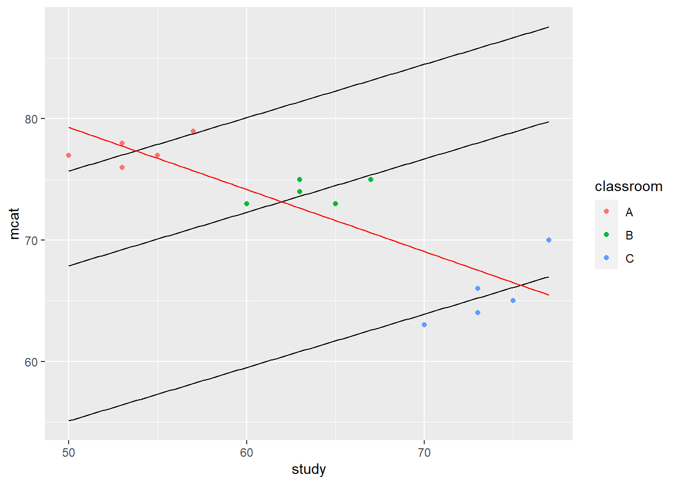

As you can see:

mcat means MCAT score percentile and is on the vertical axis. This is our outcome of interest.
study means hours spent studying and is on the horizontal axis.
We are interested in the association between mcat and study.
The students in the data are grouped into three classrooms called A, B, and C.
If we ignore that the students are grouped into classrooms, we get the incorrect, negatively-sloped red line.
If we remember that the students are grouped into classrooms and we look at the within-classroom trend, we correctly get the three correct, positively sloped black lines.

Above, students are nested within classrooms, so there are two levels of data:

Level 1	Level 2
Students	Classrooms

Nested data is also referred to as multilevel data and regression techniques to model this data are referred to collectively as multilevel modeling.

Let’s take this a step further. Imagine that we had data on students that are within classrooms that are in turn within schools. Then we would have three nested levels of data:

Level 1	Level 2	Level 3
Students	Classrooms	Schools

Each of these levels of data can have its own set of independent variables. In our previous example—with student MCAT results—we had a level 1 (student-level) independent variable which was study, and nothing else. But we hypothesized about some level 2 (classroom-level) variables.

Here are some possible independent variables for each level of our imagined data:¹⁹⁶

Level 1 – Students	Level 2 – Classrooms	Level 3 – Schools
Gender, age, number of hours spent studying, high school grade point average, mother’s education	Teacher experience, level of ambient noise, teaching style	Number of students, public/private, annual funding, average teacher salary

Previously, when we looked at MCAT performance and hours spent studying, we did not include any level 2 (classroom-level) variables in our analysis. We only looked at one level 1 (student-level) independent variable (which was hours spent studying).

This table shows what we did before:

Dependent Variable	Level 1 (student) Independent Variables	Level 2 (classroom) Independent Variables
MCAT score percentile	Hours spent studying	None

When we did our fixed effects regressions, we told the computer to control for classroom groups, but we did not tell it any characteristics (variables) of each classroom. We only told it a characteristic of the individual students (the hours they spent studying). Now, that will change, as you will see in the next section.

Before we move on, note that we will not discuss data that has even more than three levels of nesting, but you should be aware that such nesting can very plausibly be found in certain complex datasets. For example, you may have data on students within classrooms within schools within districts within states within countries. That’s six levels total! In practice, we might not often use such complex models, but it would theoretically be possible to make one if we had data that were structured like this.

11.2 Random effects models

Just like fixed effects models, which we learned about already, random effects models are another powerful tool for modeling clustered and/or nested data. Previously, with fixed effects models, we created varying intercepts and varying slopes models. Below, we will begin our study of random effects models by replicating the same varying intercepts and varying slopes models that we made before. Then we will learn more about the unique capabilities of random effects modeling.

As always, before we can trust the results of a random effects regression model, we have to make sure that the model passes all diagnostic tests of model assumptions. The diagnostics process for random effects models is not presented in this chapter, but references to resources that include this information are given.

11.2.1 Random intercepts model – replication

When we were using fixed effects before, once we realized that we had to look separately at each classroom, we first created a “varying intercepts” model using fixed effects regression. Now, we will again create a varying intercepts model, but using a different approach called random intercepts (a type of random effects modeling). The goal of this is the same: to create a model in which the observations within each group get their own regression line, such that each group’s regression line has the same slope but a unique intercept.

Let’s return to the very same practice dataset we used before. We can run the following code to load this dataset, called prep. Note that an additional variable, tqual, has been added, although we will ignore it at first.

study <- c(50,53,55,53,57,60,63,65,63,67,70,73,75,73,77)
mcat <- c(77,76,77,78,79,73,74,73,75,75,63,64,65,66,70)
classroom <- c("A","A","A","A","A","B","B","B","B","B","C","C","C","C","C")
tqual <- c(8,8,8,8,8,7,7,7,7,7,2,2,2,2,2)

prep <- data.frame(study, mcat, classroom, tqual)

Let’s begin by creating a copy of the varying intercepts model that we made before. As a reminder, here are the key variables:

Dependent variable – mcat. This is the MCAT score of each sampled pre-medical student, given as a percentile, meaning that it is on a scale from 0 to 100.
Independent variable – study. This is the number of hours that a student spent studying for the MCAT.
Group variable – classroom. This is a factor (categorical) variable that tells us which classroom each student is in.

To make a random intercepts model, we will use the lmer() function from the lme4 package in R:

if (!require(lme4)) install.packages('lme4')

## Warning: package 'lme4' was built under R version 4.2.3

## Warning: package 'Matrix' was built under R version 4.2.3

library(lme4)

randint1 <- lmer(mcat ~ study + (1|classroom), data = prep)

Here’s what the code above does:

randint1 – This is the name of the saved regression result object, just like we have saved results before with lm(...) or glm(...)
lmer() – This is just like the lm() command that we used before. This tells R that we want to make a linear mixed effects model.
mcat ~ – Like always, this tells the computer that mcat is our dependent variable.
study – Like always, this tells the computer that study is our independent variable. More could be added here, but for now there’s just this one independent variable.
(1|classroom) – This is new. This is how random effects are specified. Variables for which we want varying slopes (which we do not want at the moment) go to the left of the | symbol and the grouping variable goes to the right of the | symbol. The 1 you see to the left of the | symbol just means that we only want varying intercepts in this model, no varying slopes for any variables. In R, the number 1 means “intercept”. The classroom to the right of the | symbol tells the computer that the groups into which our observations are sorted are identified in the classroom variable.
data = prep – This is the same as always. This tells the computer that the data we want to use for this regression come from the prep dataset.

Now we can use the familiar summary(...) function to view the results:

summary(randint1)

## Linear mixed model fit by REML ['lmerMod']
## Formula: mcat ~ study + (1 | classroom)
##    Data: prep
## 
## REML criterion at convergence: 64.4
## 
## Scaled residuals: 
##     Min      1Q  Median      3Q     Max 
## -1.0756 -0.8092  0.1688  0.5104  2.1085 
## 
## Random effects:
##  Groups    Name        Variance Std.Dev.
##  classroom (Intercept) 100.533  10.027  
##  Residual                2.056   1.434  
## Number of obs: 15, groups:  classroom, 3
## 
## Fixed effects:
##             Estimate Std. Error t value
## (Intercept)  47.3928    11.4333   4.145
## study         0.3921     0.1549   2.531
## 
## Correlation of Fixed Effects:
##       (Intr)
## study -0.862

The summary regression table above is pretty complicated. We will return to it later, but for now, let’s look at a more simple output below that will show us what we need to see initially:

coef(randint1)

## $classroom
##   (Intercept)     study
## A    56.34431 0.3921469
## B    49.05267 0.3921469
## C    36.78139 0.3921469
## 
## attr(,"class")
## [1] "coef.mer"

This output from the coef(...) function gives us a slope and intercept for each classroom. We can use this information to make a separate regression equation for each classroom:

Classroom A: \(\hat{mcat} = 0.392*study + 56.34\)
Classroom B: \(\hat{mcat} = 0.392*study + 49.05\)
Classroom C: \(\hat{mcat} = 0.392*study + 36.78\)

Above are the equations for each classroom based on a random intercepts model. You’ll see that the slope of 0.392 is identical for all classrooms. You can see that it is also given in the summary table above in the row for the coefficient of study.

We can compare the random intercepts model results above to the analogous three regression equations that we saw in the previously for each classroom when we ran a varying intercepts fixed effects regression. Below are the equations for each classroom based on a fixed effects model.

Classroom A: \(\hat{mcat} = 0.441*study + 53.75\)
Classroom B: \(\hat{mcat} = 0.441*study + 45.94\)
Classroom C: \(\hat{mcat} = 0.441*study + 33.13\)

In both the random intercepts and fixed effects models, the slopes are the same for each classroom: all three slopes are 0.392 for the random intercepts equations and all three slopes are 0.441 for the fixed effects equations. This is by design. Remember: we deliberately asked the computer to look for three parallel lines, one line per classroom. For the three lines to be parallel, they all three have the same slope but have different intercepts.

You might have noticed that the results for the random intercepts model and fixed effects model above are not the same. The slope is lower and the intercepts are higher in the random effects model. This is because different estimation techniques are being used to fit the data in each model. Later, we can look at how to compare the two models to decide which is the best model to use. For now, just remember that both are trying to accomplish the same goal (to fit a model to the data with a separate intercept but the same slope for each group).

11.2.1.1 Possible error when using lme4 package and lmer models

Previously, other users of this book have encountered errors while trying to run lmer models for the first time. If you get an error, please try the following steps:

Close RStudio (first save all of your work in RMD or other files)
Open RStudio again
In the console (not in your RMD file), run: update.packages(ask = FALSE)
If you are asked if you want to install the packages in a personal library, choose YES.
Wait for the process to finish. If you get an error, email your instructors. If there are no errors, restart RStudio.
Try to run your lmer code again.

If that doesn’t work, try this:

Run detach("package:lme4", unload = TRUE)
Run detach("package:Matrix", unload = TRUE)
Run install.packages("Matrix")
Run library(lme4)
Try to run your lmer code again.

If neither of the options above work, contact your instructors immediately.

11.2.2 Random slopes model – Replication

In the previous section, we allowed our regression model to have unique intercepts for each classroom in our data, but we required that the slope be the same for all classrooms.

Previously, we made a fixed effects model in which we added interaction terms between study and classroom to create a “varying slopes” model in which each classroom had its own unique slope. In other words, the predicted association between mcat and study was allowed to be different for each classroom.

The graph below should refresh your memory about this varying slopes model:

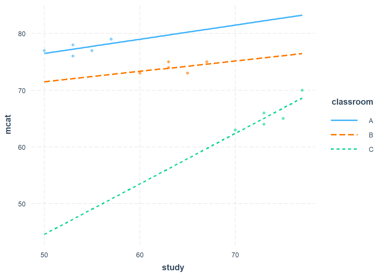
We created the model pictured above by interacting each classroom fixed effect (dummy variable) with the study variable. As you can see, the slope between mcat and study varies between classrooms (because the slope is a different steepness for each of the three classrooms). Below, we will create a similar varying intercepts model with what is called a random slopes model.

As in the previous section, we will again use the lmer() function to do this:

randslope1 <- lmer(mcat ~ study + (1+study|classroom), data = prep)

## boundary (singular) fit: see help('isSingular')

summary(randslope1)

## Linear mixed model fit by REML ['lmerMod']
## Formula: mcat ~ study + (1 + study | classroom)
##    Data: prep
## 
## REML criterion at convergence: 60.4
## 
## Scaled residuals: 
##      Min       1Q   Median       3Q      Max 
## -1.51891 -0.71487  0.06621  0.67386  1.34882 
## 
## Random effects:
##  Groups    Name        Variance  Std.Dev. Corr 
##  classroom (Intercept) 1193.2452 34.5434       
##            study          0.1352  0.3677  -1.00
##  Residual                 1.3674  1.1694       
## Number of obs: 15, groups:  classroom, 3
## 
## Fixed effects:
##             Estimate Std. Error t value
## (Intercept)  44.0786    21.5254   2.048
## study         0.4076     0.2453   1.662
## 
## Correlation of Fixed Effects:
##       (Intr)
## study -0.990
## optimizer (nloptwrap) convergence code: 0 (OK)
## boundary (singular) fit: see help('isSingular')

What we did above is very similar to what we did to estimate the random intercepts model earlier. Here are the key differences:

randslope1 – This is the name of the regression object we saved.
(1+study|classroom) – This is telling the computer that we want a random (varying) slope estimate for the study variable for each level of classroom. We keep the number 1 in there to tell the computer that we also want a random intercept. If we wanted to, we could add more than just the study variable to the left of the | symbol. For example, we could have written: (1+study+AnotherVariable+AnotherVariable2|classroom).

Again, rather than looking at the complicated summary table, let’s use the coef(...) function to look only at the estimated slope and intercept for each classroom:

coef(randslope1)

## $classroom
##   (Intercept)     study
## A    70.72531 0.1239454
## B    56.48060 0.2755825
## C     5.02994 0.8232830
## 
## attr(,"class")
## [1] "coef.mer"

Since this is a “varying slopes” model (more specifically a random slopes model), the slopes above are different for each classroom, unlike in our random intercepts model before.

Let’s plot these three lines against our data:

if (!require(dplyr)) install.packages('dplyr') 
library(dplyr)

if (!require(ggplot2)) install.packages('ggplot2') 
library(ggplot2)

p <- prep %>% ggplot(aes(study,mcat)) 

eqA = function(x){70.72 + 0.12*x}
eqB = function(x){56.48 + 0.28*x}
eqC = function(x){5.02 + 0.82*x}
p + 
  geom_point(aes(col = classroom)) + 
  stat_function(fun=eqA) + 
  stat_function(fun=eqB) + 
  stat_function(fun=eqC) +
  theme(legend.background = element_rect(fill = "transparent"))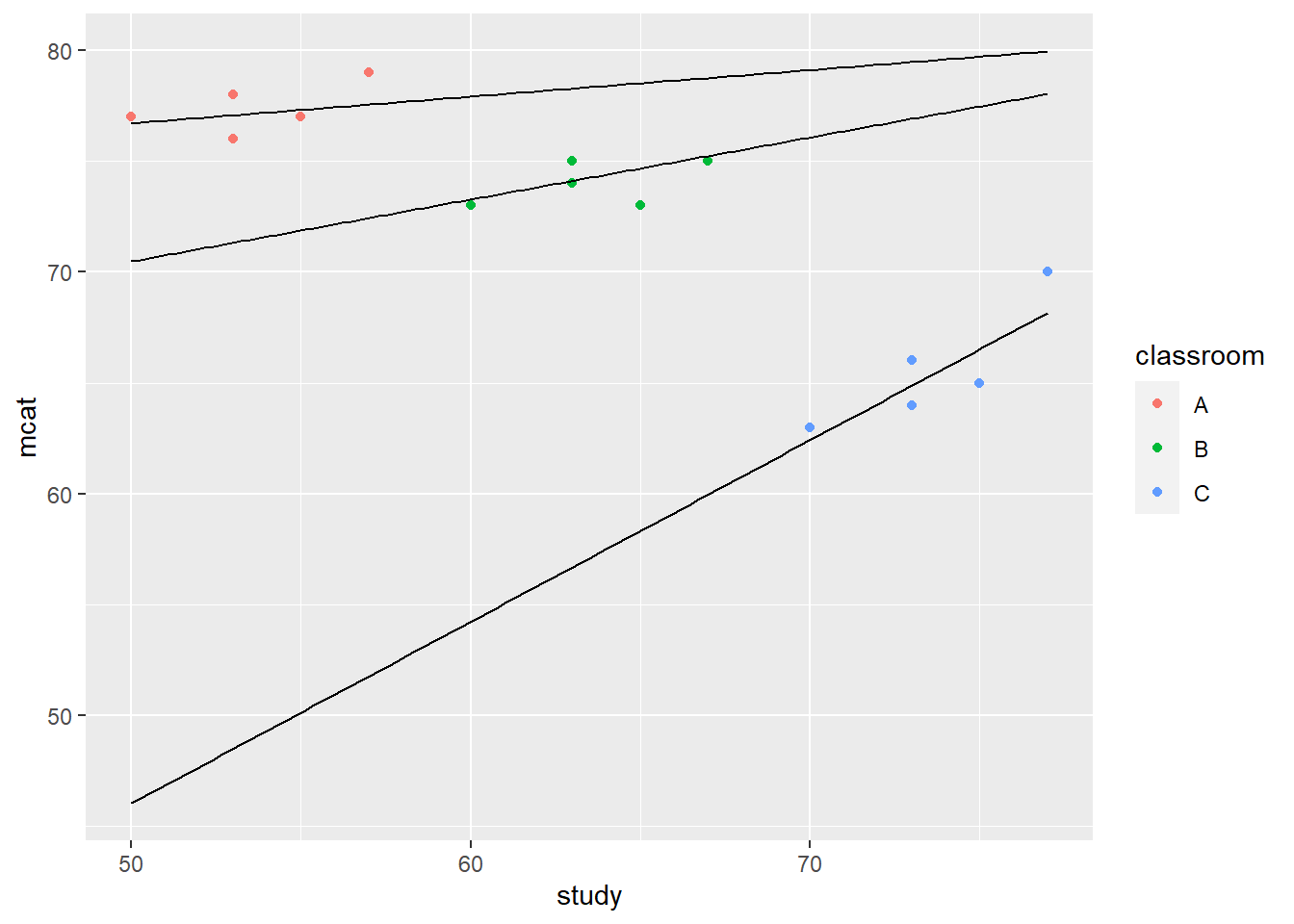

As you can see above, the regression lines appear to fit our data pretty well.

So now you know two ways to fit a varying intercepts model when you have data that is grouped:

You can run an OLS regression using the lm() command with fixed effects at the group level and interact the group variable with your independent variable of interest (as we did previously).
You can run a random slopes model using the lmer() command in which you add a parenthetical term like this: (1 + VariableOfInterest | GroupVariable). The model will then calculate a slope and intercept of the relationship between the dependent variable and your independent variable of interest separately for each group.

Now that we have run both a random intercepts and random slopes model using random effects modeling with the lmer() function, let’s look more carefully at the summary output we get.

11.2.3 `lmer()` summary output

In the random intercepts and random slopes models we looked at in the previous sections, we used the coef() function to get just the estimates we wanted for each of the three classrooms. We ignored the summary table. But now we are going to look carefully at a few parts of the summary table, because it contains a lot of important information.

Let’s look together at the summary output of the random slopes model randslope1 that we had created before:

summary(randslope1)

## Linear mixed model fit by REML ['lmerMod']
## Formula: mcat ~ study + (1 + study | classroom)
##    Data: prep
## 
## REML criterion at convergence: 60.4
## 
## Scaled residuals: 
##      Min       1Q   Median       3Q      Max 
## -1.51891 -0.71487  0.06621  0.67386  1.34882 
## 
## Random effects:
##  Groups    Name        Variance  Std.Dev. Corr 
##  classroom (Intercept) 1193.2452 34.5434       
##            study          0.1352  0.3677  -1.00
##  Residual                 1.3674  1.1694       
## Number of obs: 15, groups:  classroom, 3
## 
## Fixed effects:
##             Estimate Std. Error t value
## (Intercept)  44.0786    21.5254   2.048
## study         0.4076     0.2453   1.662
## 
## Correlation of Fixed Effects:
##       (Intr)
## study -0.990
## optimizer (nloptwrap) convergence code: 0 (OK)
## boundary (singular) fit: see help('isSingular')

We see that the results are divided into Random effects and Fixed effects sections. So, confusingly enough, random effects regression models actually have both “random” and “fixed” parts to them. We’ll get back to that later. For now, let’s just discuss how to interpret this summary output. Here are the key elements you need to know for now:

You can interpret the fixed effects portion of the output the same way you would interpret an OLS result. For every one unit increase in study, mcat is predicted to increase by 0.41. This is an average estimate of the slope across all classrooms.

The random effects portion of the output shows information related to our groups and random slopes (if there are any).
- At the bottom of this portion of the output, you can see that the computer figured out that our data has 15 observations total, divided into three classrooms.
- It then gives the variance and standard deviation for all parameters that were estimated. The variance at the group (classroom) level is 1193.2 with a standard deviation of 34.5 (the square root of the variance). 34.5 is the standard deviation of the slopes that we calculated earlier using the coef(randslope1) code earlier.
- The variance of the estimated slopes of study across all groups (classrooms) is 0.14, which corresponds to a standard deviation of 0.37. The standard deviation of the estimated slopes across all groups (classrooms) is 0.37. 0.37 is the standard deviation of the classroom level slopes of study that we saw when we ran the coef(randslope1) code earlier.

The relationship between mcat and study is predicted to be 0.41 with a standard deviation of 0.37. That’s a massive standard deviation! But it makes sense if we look at the predicted slopes and the scatterplot we made earlier. The lowest slope is 0.124 in classroom A. The highest is 0.823 in classroom C.

11.2.4 Group level variables

So far in this chapter, we have used random effects modeling to replicate what we did previously using fixed effects. We are now ready to do something new: add a classroom-level variable to our regression model. As you may have noticed when you loaded the data at the start of this chapter, a variable called tqual has now been added. tqual is a rating of teacher quality on a scale from 1–10.

Let’s have a look at the entire dataset to visually inspect this new variable, along with everything else that was there before:

prep

##    study mcat classroom tqual
## 1     50   77         A     8
## 2     53   76         A     8
## 3     55   77         A     8
## 4     53   78         A     8
## 5     57   79         A     8
## 6     60   73         B     7
## 7     63   74         B     7
## 8     65   73         B     7
## 9     63   75         B     7
## 10    67   75         B     7
## 11    70   63         C     2
## 12    73   64         C     2
## 13    75   65         C     2
## 14    73   66         C     2
## 15    77   70         C     2

As you can see above, the teacher in classroom A has quality level of 8, the teacher in classroom B has a quality level of 7, and the teacher in classroom C has a quality level of 2. Note that all students in a given classroom have the same tqual value, because tqual is a classroom-level variable. tqual is a characteristic of the classroom and not a characteristic of each individual. The power of random effects modeling is that it allows us to easily include independent variables at each level of data into our regression models.¹⁹⁷

Let’s once again use the lmer() command to run a random slopes model:

randslope2 <- lmer(mcat ~ study + tqual +  (1+study|classroom), data = prep)

## boundary (singular) fit: see help('isSingular')

To make the new regression called randslope2 above, we used the almost the exact same code as we did to make randslope1, but we added tqual as an independent variable to the non-random portion of the formula. All level 2 variables should go there. The computer knows that they are level 2 variables (group variables) automatically. Note that you could include more than just one group-level variable if you wanted.

Let’s first look at just the coefficients from this new regression we ran:

coef(randslope2)

## $classroom
##   (Intercept)     study    tqual
## A   25.730282 0.2796507 4.575312
## B   34.344241 0.1214167 4.575312
## C   -3.023588 0.8078448 4.575312
## 
## attr(,"class")
## [1] "coef.mer"

And, just for reference, let’s look at the coefficients for randslope1, which is almost the same regression but without the tqual variable included.

We can call these back any time we want like this:

coef(randslope1)

## $classroom
##   (Intercept)     study
## A    70.72531 0.1239454
## B    56.48060 0.2755825
## C     5.02994 0.8232830
## 
## attr(,"class")
## [1] "coef.mer"

The estimates in randslope1 are different than those in the newer randslope2. This is because randslope2 controls for tqual and randslope1 does not.

And now we can look at the summary table:

summary(randslope2)

## Linear mixed model fit by REML ['lmerMod']
## Formula: mcat ~ study + tqual + (1 + study | classroom)
##    Data: prep
## 
## REML criterion at convergence: 54.9
## 
## Scaled residuals: 
##     Min      1Q  Median      3Q     Max 
## -1.4407 -0.7615  0.2720  0.6605  1.4017 
## 
## Random effects:
##  Groups    Name        Variance Std.Dev. Corr 
##  classroom (Intercept) 457.2340 21.3830       
##            study         0.1543  0.3928  -1.00
##  Residual                1.4176  1.1906       
## Number of obs: 15, groups:  classroom, 3
## 
## Fixed effects:
##             Estimate Std. Error t value
## (Intercept)  19.0170    16.6781   1.140
## study         0.4030     0.2564   1.572
## tqual         4.5753     0.6683   6.846
## 
## Correlation of Fixed Effects:
##       (Intr) study 
## study -0.957       
## tqual -0.630  0.379
## optimizer (nloptwrap) convergence code: 0 (OK)
## boundary (singular) fit: see help('isSingular')

For each additional unit of teacher quality, MCAT score percentile is predicted to increase by 4.58 points! Note that this is telling us the predicted relationship between a group-level independent variable and our individual-level dependent variable.

Each additional hour of studying is associated with a predicted 0.40 increase in MCAT score percentile. This estimate has a standard deviation of 0.39.

In the next section, you’ll see how we can compare various random effects models with each other.

11.2.5 Comparing random effects models

As with logistic regression and with most other types of regression models, you will end up having to compare models that are slightly different to each other using a series of tests. As it turns out, many of the tests used to compare random effects models to each other are very similar to those used to compare logistic regression models with each other.

Earlier in this chapter, we created the following random effects models:

randint1 – A random intercepts model in which the intercepts vary across classrooms but the slope stays the same.
randslope1 – A random slopes model in which the intercepts and slopes both vary across classrooms.
randslope2 – A random slopes model in which the intercepts vary across classrooms, the slopes of the independent variable study vary across classrooms, and the variable tqual is included as a level 2 (classroom-level) independent variable.

How can we compare these models with each other to determine which one fits our data better? We will use some of the relative measures of fit that we have used before: AIC, BIC, and likelihood ratio test. We go through them one-by-one, below.

Note that we should not blindly choose the model with the best goodness-of-fit measures. We also need to consider which model is conceptually most appropriate for our data and specified correctly. Goodness-of-fit measures should only be used if we do not have a theoretical reason for choosing one model over the other. For example, if you are comparing two models—model A and model B—to each other, and model A has a lower (better) AIC but model B contains the correct variables that we need to answer our question of interest, we will still favor model B.

11.2.5.1 AIC

We previously learned about the use of the AIC statistic to measure model fit. Just like with logistic regression models, an AIC statistic can be calculated for each lmer() regression that you run. We can then compare AIC values for all of these regressions by using the following code:

AIC(randint1,randslope1,randslope2)

##            df      AIC
## randint1    4 72.42742
## randslope1  6 72.35974
## randslope2  7 68.93451

Since the lower number is better, our final model, randslope2 is the best according to the AIC comparison.

11.2.5.2 BIC

We can do the very same procedure with another goodness of fit measure called BIC, using this code:

BIC(randint1,randslope1,randslope2)

##            df      BIC
## randint1    4 75.25962
## randslope1  6 76.60804
## randslope2  7 73.89087

Like with AIC, BIC is a relative measure of model fit and lower BIC numbers also indicate better fit. According to the BIC comparison above, randslope2 fits the data the best.

11.2.5.3 Likelihood ratio test

The same likelihood ratio test that we used for logistic regression models can also be used for random effects models.

The code below runs the test on our three saved models:

if (!require(lmtest)) install.packages('lmtest')

## Warning: package 'zoo' was built under R version 4.2.3

library(lmtest)

lmtest::lrtest(randint1,randslope1,randslope2)

## Likelihood ratio test
## 
## Model 1: mcat ~ study + (1 | classroom)
## Model 2: mcat ~ study + (1 + study | classroom)
## Model 3: mcat ~ study + tqual + (1 + study | classroom)
##   #Df  LogLik Df  Chisq Pr(>Chisq)  
## 1   4 -32.214                       
## 2   6 -30.180  2 4.0677    0.13083  
## 3   7 -27.467  1 5.4252    0.01985 *
## ---
## Signif. codes:  0 '***' 0.001 '**' 0.01 '*' 0.05 '.' 0.1 ' ' 1

The result above provides some limited support for choosing model #3—randslope2—over the other two, with a p-value of 0.02.

11.2.6 Intra-class correlation (ICC)

In the example we have used so far in this chapter—with the MCAT scores and hours spent studying—it is very clear that we must use either a fixed or random effects model to account for clustered data. However, in other situations, it may not be as clear that a multilevel model of some kind is necessary.

As a first step to making a random effects model, you should always calculate what is called the intra-class correlation coefficient (ICC), which is a metric that tells us how “strongly” clustered our data is. Here is a summary from Hox et al (2018):¹⁹⁸

…multilevel models are needed because with grouped data observations from the same group are generally more similar to each other than the observations from different groups, and this violates the assumption of independence of all observations. The amount of dependence can be expressed as a correlation coefficient: the intraclass correlation.

ICC is defined as follows:¹⁹⁹

The intraclass correlation \(\rho\) indicates the proportion of the total variance explained by the grouping structure in the population.

\[\rho=\frac{\text{Variance at highest level}}{\text{Total variance}}=\frac{\text{Group variance}}{\text{Group variance}+\text{Residual Variance}}\]

How to interpret ICC:

High ICC means the data are highly clustered, meaning that results are highly dependent on the groups to which the observations belong.
Low ICC means the data are not highly (or not at all) clustered, meaning that results are not very (or not at all) dependent on the groups to which the observations belong.

To calculate ICC, we have to run an “empty” or “null” version of our regression model. We can do this with code that is the same that we have used throughout this chapter, but with all independent variables removed. Only the grouping variable and the intercepts will remain.

Note that \(\rho\) is a letter that is pronounced as “rho” and stands for “intraclass correlation.”

Here is how we begin this process using lmer():

if (!require(lme4)) install.packages('lme4')
library(lme4)

randnull <- lmer(mcat ~ 1 + (1|classroom), data = prep)
summary(randnull)

## Linear mixed model fit by REML ['lmerMod']
## Formula: mcat ~ 1 + (1 | classroom)
##    Data: prep
## 
## REML criterion at convergence: 66.8
## 
## Scaled residuals: 
##     Min      1Q  Median      3Q     Max 
## -1.5187 -0.5429 -0.1745  0.4799  2.3944 
## 
## Random effects:
##  Groups    Name        Variance Std.Dev.
##  classroom (Intercept) 36.25    6.021   
##  Residual               3.20    1.789   
## Number of obs: 15, groups:  classroom, 3
## 
## Fixed effects:
##             Estimate Std. Error t value
## (Intercept)   72.333      3.507   20.63

In the model above, we estimate random intercepts for each group in classroom. Here is what we learn from the random effects in the summary above:

Group variance = 36.25
Residual variance = 3.20

\[\rho=\frac{36.25}{36.25+3.20} = 0.919\]

This value is extremely high. This is the extent to which our data are non-independent of one another. Another way to think about this, from Hox et al (2018)²⁰⁰ is as follows:

The intraclass correlation \(\rho\) can also be interpreted as the expected correlation between two randomly drawn units that are in the same group.

In other words, \(\rho\) tells us how correlated with each other the MCAT scores from any one classroom are with each other. Imagine if we have students Aaron and Amy from classroom A; and we have students Beena and Bap from classroom B. With a high \(\rho\) as we have here, it means that Aaron and Amy’s scores are likely to be similar to each other’s; and Beena and Bap’s scores are likely to be similar to each other’s. If \(\rho\) was very low, this pattern would not exist, and the scores of Aaron, Amy, Beena, and Bap would be unrelated to each other’s scores. But, since \(\rho\) is high, we know that there is strong clustering by classroom in our data.

R has functions that can calculate ICC for us. Let’s check our math above by using the icc function from the performance package:

if (!require(performance)) install.packages('performance')

## Warning: package 'performance' was built under R version 4.2.3

library(performance)

performance::icc(randnull)

## # Intraclass Correlation Coefficient
## 
##     Adjusted ICC: 0.919
##   Unadjusted ICC: 0.919

As you can see above, our calculation was correct.

Using the summ command from the jtools package also shows the ICC, at the bottom:

if (!require(jtools)) install.packages('jtools')
library(jtools)

summ(randnull)

Observations	15
Dependent variable	mcat
Type	Mixed effects linear regression

AIC	72.83
BIC	74.96
Pseudo-R² (fixed effects)	0.00
Pseudo-R² (total)	0.92

Fixed Effects
	Est.	S.E.	t val.	d.f.	p
(Intercept)	72.33	3.51	20.63	2.00	0.00
p values calculated using Kenward-Roger standard errors and d.f.

Random Effects
Group	Parameter	Std. Dev.
classroom	(Intercept)	6.02
Residual		1.79

Grouping Variables
Group	# groups	ICC
classroom	3	0.92

When the ICC is very low, such as below 0.05 (although there is no set threshold; judgment is definitely involved as well), you may be able to run a model without random effects and still get an accurate result. However, I recommend that if your data generating mechanism is such that you might have clustered data (as is the case in educational data clustered by classrooms), you should anyway run a multilevel model because it is most appropriate to fit your data structure.

11.2.7 Inference with lmer and options to display results

You may have noticed that p-values and confidence intervals are not reported as part of the summary output for a lmer() regression object. There are a few ways around this. One is to generate confidence intervals using the confint() function that we have used before. Here is an example of how you can do that:

confint(randint1)

## Computing profile confidence intervals ...

##                   2.5 %    97.5 %
## .sig01       3.56304868 24.171453
## .sigma       0.96646135  2.235322
## (Intercept) 25.26936144 75.056993
## study       -0.03690402  0.687023

Another very popular and useful package is called stargazer. You can install it and then use it as follows:

if (!require(stargazer)) install.packages('stargazer')
library(stargazer)

stargazer(randslope2, type = "text", ci=TRUE)

## 
## ===============================================
##                         Dependent variable:    
##                     ---------------------------
##                                mcat            
## -----------------------------------------------
## study                          0.403           
##                           (-0.100, 0.905)      
##                                                
## tqual                        4.575***          
##                           (3.266, 5.885)       
##                                                
## Constant                      19.017           
##                          (-13.671, 51.705)     
##                                                
## -----------------------------------------------
## Observations                    15             
## Log Likelihood                -27.467          
## Akaike Inf. Crit.             68.935           
## Bayesian Inf. Crit.           73.891           
## ===============================================
## Note:               *p<0.1; **p<0.05; ***p<0.01

You can also have stargazer display the results of multiple models side-by-side by using the following code (the result is not displayed):

stargazer(randint1, randslope1, randslope2, type = "text", ci=TRUE)

## 
## ======================================================================
##                                    Dependent variable:                
##                     --------------------------------------------------
##                                            mcat                       
##                           (1)              (2)              (3)       
## ----------------------------------------------------------------------
## study                   0.392**          0.408*            0.403      
##                      (0.089, 0.696)  (-0.073, 0.888)  (-0.100, 0.905) 
##                                                                       
## tqual                                                    4.575***     
##                                                       (3.266, 5.885)  
##                                                                       
## Constant               47.393***        44.079**          19.017      
##                     (24.984, 69.802) (1.890, 86.268) (-13.671, 51.705)
##                                                                       
## ----------------------------------------------------------------------
## Observations               15              15               15        
## Log Likelihood          -32.214          -30.180          -27.467     
## Akaike Inf. Crit.        72.427          72.360           68.935      
## Bayesian Inf. Crit.      75.260          76.608           73.891      
## ======================================================================
## Note:                                      *p<0.1; **p<0.05; ***p<0.01

Note that you can change the type = argument to 'html' if you are knitting an HTML file or to 'latex' if you are making a PDF, and it should output an even nicer-looking table.

Note that while stargazer will show the fixed effect estimates and the confidence intervals, it does not show the random effects portion of the results.

Another option is to install and load the jtools package and then run the following code:

if (!require(jtools)) install.packages('jtools')
library(jtools)

summ(randslope2, confint=TRUE)

Observations	15
Dependent variable	mcat
Type	Mixed effects linear regression

AIC	68.93
BIC	73.89
Pseudo-R² (fixed effects)	0.78
Pseudo-R² (total)	0.99

Fixed Effects
	Est.	2.5%	97.5%	t val.	d.f.	p
(Intercept)	19.02	-13.67	51.71	1.06	3.44	0.36
study	0.40	-0.10	0.91	1.37	1.99	0.30
tqual	4.58	3.27	5.89	4.05	4.57	0.01
p values calculated using Kenward-Roger standard errors and d.f.

Random Effects
Group	Parameter	Std. Dev.
classroom	(Intercept)	21.38
classroom	study	0.39
Residual		1.19

Grouping Variables
Group	# groups	ICC
classroom	3	1.00

This output, above, gives the same confidence intervals as stargazer, but it calculates the p-values differently. However, it does include the random effects portion of the output.

Finally, here is another option, from the package sjPlot, which only works for HTML output but does give a quite nice table including both fixed and random effects:

if (!require(sjPlot)) install.packages('sjPlot')
library(sjPlot)

tab_model(randslope2)

Ultimately, it is more important for you to look at the confidence intervals for each estimate rather than the p-values.

11.2.8 Resolving errors (optional)

This section is completely optional (not required) to read and learn. You will not be required to know anything in this section for any homeworks or oral exams.

Below, we will explore a few common errors that you might come across while running random effects models.

11.2.8.1 Singular fit

In the model randslope2 that we ran earlier in this chapter, we got the following error message:

boundary (singular) fit: see ?isSingular

This indicates that we have a problem due to what is called singularity in our regression model. The following two paragraphs from the Princeton University Library summarize what this means and relates it to a concept that you are already familiar with—multicollinearity:²⁰¹

Multicollinearity is a condition in which the IVs are very highly correlated (.90 or greater) and singularity is when the IVs are perfectly correlated and one IV is a combination of one or more of the other IVs. Multicollinearity and singularity can be caused by high bivariate correlations (usually of .90 or greater) or by high multivariate correlations. High bivariate correlations are easy to spot by simply running correlations among your IVs. If you do have high bivariate correlations, your problem is easily solved by deleting one of the two variables, but you should check your programming first, often this is a mistake when you created the variables. It’s harder to spot high multivariate correlations. To do this, you need to calculate the SMC for each IV. SMC is the squared multiple correlation ( R2 ) of the IV when it serves as the DV which is predicted by the rest of the IVs. Tolerance, a related concept, is calculated by 1-SMC. Tolerance is the proportion of a variable’s variance that is not accounted for by the other IVs in the equation. You don’t need to worry too much about tolerance in that most programs will not allow a variable to enter the regression model if tolerance is too low.

Statistically, you do not want singularity or multicollinearity because calculation of the regression coefficients is done through matrix inversion. Consequently, if singularity exists, the inversion is impossible, and if multicollinearity exists the inversion is unstable. Logically, you don’t want multicollinearity or singularity because if they exist, then your IVs are redundant with one another. In such a case, one IV doesn’t add any predictive value over another IV, but you do lose a degree of freedom. As such, having multicollinearity/ singularity can weaken your analysis. In general, you probably wouldn’t want to include two IVs that correlate with one another at .70 or greater.

Let’s again review the regression table that we saw earlier in the chapter:

randslope2 <- lmer(mcat ~ study + tqual +  (1+study|classroom), data = prep)

## boundary (singular) fit: see help('isSingular')

summary(randslope2)

## Linear mixed model fit by REML ['lmerMod']
## Formula: mcat ~ study + tqual + (1 + study | classroom)
##    Data: prep
## 
## REML criterion at convergence: 54.9
## 
## Scaled residuals: 
##     Min      1Q  Median      3Q     Max 
## -1.4407 -0.7615  0.2720  0.6605  1.4017 
## 
## Random effects:
##  Groups    Name        Variance Std.Dev. Corr 
##  classroom (Intercept) 457.2340 21.3830       
##            study         0.1543  0.3928  -1.00
##  Residual                1.4176  1.1906       
## Number of obs: 15, groups:  classroom, 3
## 
## Fixed effects:
##             Estimate Std. Error t value
## (Intercept)  19.0170    16.6781   1.140
## study         0.4030     0.2564   1.572
## tqual         4.5753     0.6683   6.846
## 
## Correlation of Fixed Effects:
##       (Intr) study 
## study -0.957       
## tqual -0.630  0.379
## optimizer (nloptwrap) convergence code: 0 (OK)
## boundary (singular) fit: see help('isSingular')

As you can see, we get the error message boundary (singular) fit: see ?isSingular

To read more about this issue from within R, type ?lme4::isSingular into the console.²⁰² Below are some of the key points, copied from the longer explanation that you will see:

There is not yet consensus about how to deal with singularity, or more generally to choose which random-effects specification (from a range of choices of varying complexity) to use. Some proposals include:

avoid fitting overly complex models in the first place, i.e. design experiments/restrict models a priori such that the variance-covariance matrices can be estimated precisely enough to avoid singularity (Matuschek et al 2017)
use some form of model selection to choose a model that balances predictive accuracy and overfitting/type I error (Bates et al 2015, Matuschek et al 2017)
“keep it maximal”, i.e. fit the most complex model consistent with the experimental design, removing only terms required to allow a non-singular fit (Barr et al. 2013), or removing further terms based on p-values or AIC
use a partially Bayesian method that produces maximum a posteriori (MAP) estimates using regularizing priors to force the estimated random-effects variance-covariance matrices away from singularity (Chung et al 2013, blme package)
use a fully Bayesian method that both regularizes the model via informative priors and gives estimates and credible intervals for all parameters that average over the uncertainty in the random effects parameters (Gelman and Hill 2006, McElreath 2015; MCMCglmm, rstanarm and brms packages)

The italicized text above comes directly from the explanation you should see if you run the command ?lme4::isSingular in the console.

Below, you’ll see an attempt to run the same model using the blme package that was mentioned above:

if (!require(blme)) install.packages('blme')
library(blme)

randslope2a <- blmer(mcat ~ study + tqual +  (1+study|classroom), data = prep, REML = TRUE)

## Warning in checkConv(attr(opt, "derivs"), opt$par, ctrl = control$checkConv, :
## unable to evaluate scaled gradient

## Warning in checkConv(attr(opt, "derivs"), opt$par, ctrl = control$checkConv, :
## Model failed to converge: degenerate Hessian with 1 negative eigenvalues

Note that we used the blmer() function from the blme package, instead of the lmer() function from the lme4 package. Above, we do not have a “singular fit” problem anymore, but we do have a new problem related to convergence. We get the following error:

Model failed to converge with max|grad| = 0.00411774 (tol = 0.002, component 1)

Continue on to the next section to see one possible way to address this problem!

11.2.8.2 Convergence

Sometimes you may see an error that indicates that the lmer() model you ran did not converge. This can be due to a number of reasons which we will not fully explore in this section. One problem could simply be that the sample size in your data or in each group in your data is not large enough. Another issue can be that the optimization procedure that the computer used to fit the model was not able to fully or successfully fit the model.

A possible solution can be to try using a different optimization procedure to fit the data. An example of this procedure is below, and you can try using this code if you also run into an error.

Let’s start by re-running the random effects model we used earlier in this chapter:

randslope2 <- lmer(mcat ~ study + tqual +  (1+study|classroom), data = prep)

## boundary (singular) fit: see help('isSingular')

summary(randslope2)

## Linear mixed model fit by REML ['lmerMod']
## Formula: mcat ~ study + tqual + (1 + study | classroom)
##    Data: prep
## 
## REML criterion at convergence: 54.9
## 
## Scaled residuals: 
##     Min      1Q  Median      3Q     Max 
## -1.4407 -0.7615  0.2720  0.6605  1.4017 
## 
## Random effects:
##  Groups    Name        Variance Std.Dev. Corr 
##  classroom (Intercept) 457.2340 21.3830       
##            study         0.1543  0.3928  -1.00
##  Residual                1.4176  1.1906       
## Number of obs: 15, groups:  classroom, 3
## 
## Fixed effects:
##             Estimate Std. Error t value
## (Intercept)  19.0170    16.6781   1.140
## study         0.4030     0.2564   1.572
## tqual         4.5753     0.6683   6.846
## 
## Correlation of Fixed Effects:
##       (Intr) study 
## study -0.957       
## tqual -0.630  0.379
## optimizer (nloptwrap) convergence code: 0 (OK)
## boundary (singular) fit: see help('isSingular')

Now, even though there wasn’t an error in the output above, let’s imagine that there was an error and what we would do about it. Here is an example of a common error message that you might see:

Model failed to converge with max|grad| = 0.0179593 (tol = 0.002, component 1)

If you see an error like that, you can try to re-run your regression model a second time, using some information we have from the initial model. In this case, the initial model was randslope2, above. Below, we’ll extract some information from this model:

ss <- getME(randslope2,c("theta","fixef"))

Above, we have stored some information from randslope2 as the variable ss. Next, we will run our regression once again, creating model randslope2b:

randslope2b <- lmer(mcat ~ study + tqual +  (1+study|classroom), data = prep, start=ss, control=lmerControl(optimizer="bobyqa", optCtrl=list(maxfun=2e5)))

## boundary (singular) fit: see help('isSingular')

summary(randslope2b)

## Linear mixed model fit by REML ['lmerMod']
## Formula: mcat ~ study + tqual + (1 + study | classroom)
##    Data: prep
## Control: lmerControl(optimizer = "bobyqa", optCtrl = list(maxfun = 2e+05))
## 
## REML criterion at convergence: 54.9
## 
## Scaled residuals: 
##     Min      1Q  Median      3Q     Max 
## -1.4407 -0.7615  0.2720  0.6605  1.4017 
## 
## Random effects:
##  Groups    Name        Variance Std.Dev. Corr 
##  classroom (Intercept) 457.2340 21.3830       
##            study         0.1543  0.3928  -1.00
##  Residual                1.4176  1.1906       
## Number of obs: 15, groups:  classroom, 3
## 
## Fixed effects:
##             Estimate Std. Error t value
## (Intercept)  19.0170    16.6781   1.140
## study         0.4030     0.2564   1.572
## tqual         4.5753     0.6683   6.846
## 
## Correlation of Fixed Effects:
##       (Intr) study 
## study -0.957       
## tqual -0.630  0.379
## optimizer (bobyqa) convergence code: 0 (OK)
## boundary (singular) fit: see help('isSingular')

Now, the convergence error may have gone away. This is because we used a different optimization strategy. You can try this approach if you are having the same problem. The singular fit error is still there in randslope2b, however. If we were using this data for real research (instead of practice as we are now), we would want to use a model that resolved both of the issues before trusting the results we found.

The following resources can be consulted for further information about resolving issues related to convergence:

The strategy demonstrated above in this chapter was adapted from these resources listed above.

In the previous section about singular fit, we saw how to resolve the singular fit issue, but then we had a convergence error (see model randslope2a). Let’s try and fix that error, below, using the same procedure that was just demonstrated above:

ss <- getME(randslope2a,c("theta"))

randslope2c <- blmer(mcat ~ study + tqual +  (1+study|classroom), data = prep, REML = TRUE, start=ss, control=lmerControl(optimizer="bobyqa", optCtrl=list(maxfun=2e5)))
summary(randslope2c)

## Cov prior  : classroom ~ wishart(df = 4.5, scale = Inf, posterior.scale = cov, common.scale = TRUE)
## Prior dev  : -25.0359
## 
## Linear mixed model fit by REML ['blmerMod']
## Formula: mcat ~ study + tqual + (1 + study | classroom)
##    Data: prep
## Control: lmerControl(optimizer = "bobyqa", optCtrl = list(maxfun = 2e+05))
## 
## REML criterion at convergence: 72.8
## 
## Scaled residuals: 
##     Min      1Q  Median      3Q     Max 
## -1.6309 -0.8337  0.2909  0.6621  1.3230 
## 
## Random effects:
##  Groups    Name        Variance  Std.Dev.  Corr
##  classroom (Intercept) 3.785e+07 6152.6065     
##            study       7.072e-01    0.8409 0.00
##  Residual              1.229e+00    1.1085     
## Number of obs: 15, groups:  classroom, 3
## 
## Fixed effects:
##              Estimate Std. Error t value
## (Intercept)  -13.4857  8451.9553  -0.002
## study          0.4412     0.5008   0.881
## tqual          9.8393  1353.3952   0.007
## 
## Correlation of Fixed Effects:
##       (Intr) study 
## study -0.001       
## tqual -0.907  0.000

In the version above, you’ll see that we finally managed to run a model without getting any error messages. If you want, you can compare the results we got from randslope2, randslope2a, randslope2b, and randslope2c to each other to see how different or similar they are.

It is important to remember that the approaches demonstrated above are not the ONLY way to fix problems with your random effects model. They are only one method that you can attempt.

11.2.9 Optional resources

If you wish to read more about multilevel modeling, the following resources may be useful. They also include additional examples that could be good supplements to the example you saw above in this chapter. Please keep in mind that you are not required to read any of these. They are just here for additional reference if needed.

Chapter 2 in J.J. Hox, M. Moerbeek & R. van de Schoot (2018). Multilevel Analysis. Techniques and Applications. New York, NY: Routledge. https://multilevel-analysis.sites.uu.nl/wp-content/uploads/sites/27/2018/02/02Ch2-Basic3449.pdf
Starkweather, J. Linear Mixed Effects Modeling using R. http://bayes.acs.unt.edu:8083/BayesContent/class/Jon/Benchmarks/LinearMixedModels_JDS_Dec2010.pdf.
Knowles, J. 2013. Getting Started with Mixed Effect Models in R. https://www.jaredknowles.com/journal/2013/11/25/getting-started-with-mixed-effect-models-in-r.
Smeeets, L & van de Schoot, R. 2019. LME4 Tutorial: Popularity Data. https://www.rensvandeschoot.com/tutorials/lme4/.
Bates, D et al. Fitting Linear Mixed-Effects Models Using lme4. https://cran.r-project.org/web/packages/lme4/vignettes/lmer.pdf.

11.3 Assignment

In this chapter’s assignment, you will return to the data you used in the previous assignment on fixed effects models. You will start by running an ICC calculation. Then, you will run the same analysis as before, but this time you will use random effects models from the lme4 package and use the lmer() function, as demonstrated throughout this chapter. Finally, you will run additional models with additional variables included, to see how this changes your estimates.

To refresh your memory, please read the following description of this data:²⁰³

The GALO data in file galo are from an educational study by Schijf and Dronkers (1991). They are data from 1377 pupils within 58 schools. We have the following pupil-level variables: father’s occupational status, focc; father’s education, feduc; mother’s education, meduc; pupil sex, sex; the result of GALO school achievement test, GALO; and the teacher’s advice about secondary education, advice. At the school level we have only one variable: the school’s denomination, denom. Denomination is coded 1 = Protestant, 2 = nondenominational, 3 = Catholic (categories based on optimal scaling).

If you don’t still have it saved on your computer, please click here to download the data again for the assignment below. Click on the Download button at this page to download the dataset called GaloComplete.sav.

Next, use this exact code to load the data and recode some of the variables:

if (!require(foreign)) install.packages('foreign')
library(foreign)

df <- read.spss("GaloComplete.sav", to.data.frame = TRUE)
df$meduc <- as.numeric(df$meduc)
df$school <- as.factor(df$school)

Remember that you are investigating the following question of interest: What is the relationship between mother’s education (independent variable) and GALO score (dependent variable)?

Other reminders and instructions from the previous assignment on fixed effects models once again apply to this assignment. Please take a moment to go back and review those before you start the assignment below.

11.3.1 ICC

Even though ICC was presented towards the end of the reading in this chapter, it’s actually what you should do at the very start of an analysis. So we’re going to start with ICC in this assignment.

Task 1: Make a null model for your research question, using the lmer() function. If you get an error message when trying to make this model, try the steps below.

To resolve an lmer error, try this:

Close RStudio (first save all of your work in RMD or other files)
Open RStudio again
In the console (not in your RMD file), run: update.packages(ask = FALSE)
If you are asked if you want to install the packages in a personal library, choose YES.
Wait for the process to finish. If you get an error, email your instructors. If there are no errors, restart RStudio.
Try to run your lmer code again.

If that doesn’t work, try this:

Run detach("package:lme4", unload = TRUE)
Run detach("package:Matrix", unload = TRUE)
Run install.packages("Matrix")
Run library(lme4)
Try to run your lmer code again.

If neither of the options above work, contact your instructors immediately.

Task 2: Calculate the ICC “by hand”, meaning that you should show the calculation as a fraction and then the answer.

Task 3: Have R calculate the ICC for you to verify that you did it correctly in the previous task. Show your code and the result.

Task 4: Interpret the ICC that you found.

11.3.2 Random intercepts model

In this part of the assignment, you will replicate what you did previously with fixed effects, creating a varying-intercepts (but constant slope) model using the random intercepts method with lmer(...) that was demonstrated earlier in this chapter.

Task 5: Run and interpret a random intercepts model to answer the question of interest. Use the same dependent and independent variables as you used in the fixed effects assignment that you did previously (from the final regression model that you made in that assignment). Use galo as the dependent variable and meduc as the independent variable. This will be called Model 1. Display the appropriate summary table(s) and give a sample and population level interpretation of the results.

Task 6: Compare your fixed effects model from the fixed effects assignment to the random intercepts model—called Model 1—that you just made. How are the results similar or different?

11.3.3 Random slopes model

In this part of the assignment, you will replicate the varying-slopes model that you created with fixed effects models before, this time using a random slopes model with lmer() as demonstrated in this chapter.

Task 7: Run and interpret a random slopes model that is analogous to the “varying-slopes model” that you ran in the fixed effects assignment. The dependent and independent variables should be exactly the same, but the way you specify the model will of course be different. This will be called Model 2. Display the appropriate summary table(s) and give a sample and population level interpretation of the results.

Note that you might get a warning such as Warning in checkconv... and/or Model failed to converge with max|grad|.... In our class, we don’t have time to fully address this error. Please just proceed to interpret the results as if this error did not appear. However, if you do want to debug this issue, you can try the steps suggested earlier in this chapter.

Task 8: Compare your varying-slopes model from the fixed effects assignment to the random slopes model—called Model 2—that you just made. How are the results similar or different?

11.3.4 Add additional variables

Now, finally, we will do something brand new that we did not do in the fixed effects assignment before. In this part of the assignment, you will add a group-level variable into your analysis, again using the lmer() function. You will also add in a control variable at the individual level.

Task 9: Add in the variable denom as a school-level variable and run a third lmer model. This will be called Model 3. Show and interpret the results for both sample and population. Only run a random slopes model, not random intercepts. You will have random slopes for meduc that vary from school to school, not for denom. denom will have a fixed slope that doesn’t vary from school to school.

Task 10: Add in sex as an individual-level control variable. Show and interpret the results. This will be called Model 4. Only run a random slopes model; not random intercepts. You will NOT have random slopes for sex and denom. You WILL still have random slopes for meduc.

11.3.5 Comparing models

As you’ll find as you do more independent quantitative analysis of your own, much of your time will be spent comparing different regression models to each other to figure out which one is the best suited for your data and question. In this part of the assignment, you will practice comparing various regression models with each other.

Task 11: Compare all four regression models that you have created in this assignment to each other. Which one is the best? Use at least two methods of comparison that were demonstrated in this chapter. Also provide a theoretical justification for choosing one model over the rest. Be sure to show all of your code, results, and written interpretation.

11.3.6 Additional items

You have now reached the end of this week’s assignment. The tasks below will guide you through submission of the assignment, remind you of any other items you need to complete this week, and allow us to gather questions and/or feedback from you.

Task 12: You are required to complete 15 quiz question flashcards in the Adaptive Learner App by the end of this week.

Task 13: Please write any questions you have for the course instructors (optional).

Task 14: Please write any feedback you have about the instructional materials (optional).

Task 15: Knit (export) your RMarkdown file into a format of your choosing.

Task 16: Please e-mail Nicole and Anshul to schedule a time for your Oral Exam #2, if you have not done so already.

Task 17: Please submit your assignment to the D2L assignment drop-box corresponding to this chapter and week of the course. And remember that if you have trouble getting your RMarkdown file to knit, you can submit your RMarkdown file itself. You can also submit an additional file(s) if needed.

Note that group-level independent variables can be included in fixed effects models; we just didn’t do this when we learned about fixed effects models.↩︎
Note that we are assuming above that each classroom always has the same teacher and that multiple teachers do not rotate through individual classrooms.↩︎
It is also possible to do this with fixed effects modeling alone, although we did not study how to do that in this textbook.↩︎
Chapter 2 in J.J. Hox, M. Moerbeek & R. van de Schoot (2018). Multilevel Analysis. Techniques and Applications. New York, NY: Routledge. https://multilevel-analysis.sites.uu.nl/wp-content/uploads/sites/27/2018/02/02Ch2-Basic3449.pdf ↩︎
Hox et al, 2018↩︎
Chapter 2 in J.J. Hox, M. Moerbeek & R. van de Schoot (2018). Multilevel Analysis. Techniques and Applications. New York, NY: Routledge. https://multilevel-analysis.sites.uu.nl/wp-content/uploads/sites/27/2018/02/02Ch2-Basic3449.pdf ↩︎
Source: Introduction to Regression ↩︎
Make sure that the lme4 package is loaded before you do this.↩︎
Source: Datasets. https://multilevel-analysis.sites.uu.nl/datasets/↩︎