Chapter 8 Causal Inference and Regression Model Specification

This week, our goals are to…

1. Use mathematical notation used to describe regression results in more detail than before.

2. Use counterfactual thinking and causal inference diagrams to improve our quantitative research design skills.

3. Practice resolving issues related to model specification such as confounding, omitted variable bias, and overfitting.

4. Begin preparation for final projects.

Announcements and reminders

1. Unlike most other weeks of our course, this week features a number of external resources that you are required to read. Much of this week’s work relates to reading you will do about the theory of quantitative analysis, rather than running analyses in R. This chapter is a break from using R but not a break from thinking hard and working hard.

2. As usual, I highly recommend that you quickly look over the assignment at the end of the chapter before you begin reading the chapter. This way, you will have a sense for which portions of each external reading correspond to each part of the assignment.

3. Please email both Nicole and Anshul to schedule your Oral Exam #2. The course calendar shows the ideal schedule for completing Oral Exam #2.

8.1 Review of sample and population results

This section contains some review and clarifications regarding sample and population results. When interpreting results from regression models, t-tests, and similar approaches, it can be easy to accidentally conclude that the result for the sample is the same as the result for your population. This is never the case.¹⁶⁵ The results reported by the analysis are always the average truth in your sample. The confidence intervals and p-values only refer to your population of interest, and they are just guesses.

Here are some examples:

1. You are running a randomized controlled trial (RCT) on whether students do better on a 20-question test after preparing for the test however they want (control group) or after following a special spaced learning protocol that you designed (treatment group). You do the experiment with a total of 100 students. You find that the control group of 50 students has a mean of 12 correctly answered questions, with a standard deviation of 4 correctly answered questions. You find that the treatment group of 50 different students has a mean of 15 correctly answered questions, with a standard deviation of 2 correctly answered questions. The answer to your research question in your sample is simply \(15-12=3 \text{ correctly answered questions}\). That’s it. It is just the difference in the means when we are talking about the sample. To answer your question in your population, you do a t-test and find that the 95% confidence interval for this difference is 1.74 to 4.26. This means that in your population of interest, you are 95% confident that your special spaced learning protocol is associated with an increased test score of at least 1.74 and at most 4.26 extra correctly answered questions on average, assuming that all t-test assumptions (diagnostic tests) are satisfied. Note that the t-test was only needed to do inference about the population; it was not needed to analyze our sample alone.

2. Now let’s say that in the scenario above, you also collect demographic information—age, sex, and domestic or foreign born status—on each of your students. Now you make a regression model in which the dependent variable is test score and there are four independent variables: dummy variables for treatment or control group, sex, and domestic or foreign status; and a continuous variable for age. You run an OLS regression model and get an estimate of 2.8 for the treatment/control dummy variable (which is coded as 1 for treatment and 0 for control). This estimate has a 95% confidence interval of 1.36 to 4.24. The answer in your sample is simply that the treatment group scores 2.8 points higher than the control group in your sample on average, controlling for age, sex, and domestic or foreign born status. That’s it. It is just the estimate (slope) alone when we are talking about the sample. When we turn to the population, that is where we look at the 95% confidence intervals, p-values, and diagnostic tests of regression assumptions. In this case, our result is that we are 95% confident that those receiving the special spaced learning protocol in our population of interest score at least 1.36 and at most 4.24 correctly answered questions higher than those in our control group on average, controlling for all other independent variables (age, sex, domestic/foreign) and assuming that all diagnostic tests of regression assumptions are passed. Note that we only used the slope estimate for our sample; the confidence intervals only relate to our population result.

8.2 Regression equation notation

In this course, we first began by writing a linear equation like this:

\[y = mx + b\]

And then we re-wrote it like this for simple linear regression:

\[\hat{y} = b_1x_1 + b_0\]

If we’re doing a regression with multiple independent variables, we can write this:

\[\hat{y} = b_1x_1 + b_2x_2 + ... + b_nx_n + b_0\]

The equation above is a general version of the equation that we can write for \(n\) (any number of) independent variables. \(b_0\) is the intercept. The other \(b\) coefficients are the slopes estimated in the regression output.

\(\hat{y}\) means the predicted value of the dependent variable according to the regression model.

Now we’ll relate these equations back to our data (whichever data was used for the regression). Let’s say that each observation in our data is a person. So our first row of data will be one person. Let’s say the person in the first row is named Mul. Mul has a specific y value (specific value of the dependent variable). Let’s call this value \(y_{Mul}\). This is the true/actual value of \(y\) (the dependent variable) for Mul. After we run a regression analysis on this data, we get a predicted value for Mul. That predicted value is \(\hat{y}_{Mul}\).

What do we usually do after we determine the actual value and the predicted value for a single person in our data? We calculate the residual. We subtract the predicted value from the actual value to get the residual. So we’re going to do the same thing here:

\[Actual\text{ }Value - Predicted\text{ }Value = Residual\]

We can rewrite the equation above like this:

\[y_{Mul} - \hat{y}_{Mul} = e_{Mul}\]

\(e_{Mul}\) is the residual for Mul, which we can also call the error. Now that we have this equation for Mul, let’s re-write this equation for anybody in our data. Let’s write \(i\) to mean anybody in the data:

\[y_i - \hat{y}_i = e_i\]

Above is how we calculate the residual for anybody—called \(i\)—in our data. Sometimes we will drop the \(i\) notation and we will simply write this:

\[y - \hat{y} = e\]

Now we’re going to add \(\hat{y}\) to both sides of the equation and we end up with this:

\[y = \hat{y} + e\]

Above, we saw that

\[\hat{y} = b_1x_1 + b_2x_2 + ... + b_nx_n + b_0\]

Let’s plug this equation above for \(\hat{y}\) into the previous equation for \(y\). The parentheses below demonstrate the plugging in process:

\[y = (\hat{y} = b_1x_1 + b_2x_2 + ... + b_nx_n + b_0) + e\]

And here’s the equation we end up with:

\[y = b_1x_1 + b_2x_2 + ... + b_nx_n + b_0 + e\]

The \(e\) is still the very same residual from earlier.

Remember, we can always rewrite this for each individual in the data. First, for our example person named Mul:

\[y_{Mul} = b_1x_{1,Mul} + b_2x_{2,Mul} + ... + b_nx_{n,Mul} + b_0 + e_{Mul}\]

If we plug in the X variable (independent variable) values from Mul’s row of data, plug in Mul’s residual, and keep the slope coefficients (the \(b\) values) the same way they are in the regression table, we will get Mul’s exact \(y\) value.

And here’s the equation for any individual, without specifying which person. We just replace \(Mul\) with \(i\):

\[y_{i} = b_1x_{1,i} + b_2x_{2,i} + ... + b_nx_{n,i} + b_0 + e_{i}\]

It is important to understand these equations for this week’s material and in the future. Being able to use these equations will enable you to better understand how to create a regression model that best fits your data and best answers your quantitative research question.

8.2.1 Summary of regression equation notation

Below is a summary of everything that you need to know related to regression equation notation as you continue to work through this chapter.

8.2.1.1 Directory of abbreviations and symbols

Actual values of the dependent variable:

• \(y\) – Actual value of the dependent variable.
• \(y_i\) – Actual value of the dependent variable for a single observation (a single row of our dataset spreadsheet).

Predicted values of the dependent variable:

• \(\hat{y}\) – Predicted value of the dependent variable.
• \(\hat{y_i}\) – Predicted value of the dependent variable for a single observation (a single row of our dataset spreadsheet).

Independent variables:

• \(x_n\) – The nth independent variable.
• \(x_{n,i}\) – The value of the nth independent variable for a single observation (a single row of our dataset spreadsheet).
• \(b_n\) – The slope coefficient for the nth independent variable.
• \(b_n\) – The slope coefficient for the nth independent variable.

Residuals:

• \(e\) – The residual error term. This represents all of the error in the regression model.
• \(e_i\) – The residual for a single observation (a single row of our dataset spreadsheet).

8.2.1.2 Important equations and their plain words translations

Actual values of the dependent variable:

• \(y-\hat{y}=e\) – Actual value minus predicted value is equal to the residual error. This can also be written as: \(y=\hat{y}+e\)
• \(y_i-\hat{y_i}=e_i\) – A single observation’s actual value minus that single observation’s predicted value is equal to that single observation’s residual. This can also be written as: \(y_i=\hat{y_i}+e_i\)

Predicted values of the dependent variable:

• \(\hat{y} = b_1x_1 + b_2x_2 + ... + b_nx_n + b_0\) – The predicted value of the dependent variable is equal to the sum of the slopes of each independent variable multiplied by each independent variable plus the intercept.
• \(\hat{y_{i}} = b_1x_{1,i} + b_2x_{2,i} + ... + b_nx_{n,i} + b_0\) – The predicted value of the dependent variable for a single observation (a single row of our dataset spreadsheet) is equal to the sum of the slopes of each independent variable multiplied by the specific values of that single observation’s independent variables plus the intercept.

Actual values of the dependent variable, again:

• \(y = b_1x_1 + b_2x_2 + ... + b_nx_n + b_0+e\) – The actual value of the dependent variable is equal to the sum of the slopes of each independent variable multiplied by each independent variable plus the intercept plus the residual error.
• \(y_{i} = b_1x_{1,i} + b_2x_{2,i} + ... + b_nx_{n,i} + b_0 + e_i\) – The actual value of the dependent variable for a single observation (a single row of our dataset spreadsheet) is equal to the sum of the slopes of each independent variable multiplied by the specific values of that single observation’s independent variables plus the intercept plus the residual of that single observation.

8.2.1.3 Example

Consider the following regression equation result which we have seen before:

\[\hat{disp} = 104.81 wt - 50.75 drat + 34.23 am + 62.14\]

Above, the predicted value of \(disp\) is equal to the formula on the right side of the equation.

We can re-write this equation for a single observation (a single row of our dataset spreadsheet):

\[\hat{disp_i} = 104.81 wt_i - 50.75 drat_i + 34.23 am_i + 62.14\]

The equation above means that if we plug in a single observation’s specific values of \(wt\), \(drat\), and \(am\) into the equation, we will get the predicted value of \(disp\) for just that observation.

Above, we looked at the equation for the predicted value of \(disp\), which we wrote as \(\hat{disp}\). Now we can also write an equation for the actual value of \(disp\).

Actual value of \(disp\):

\[disp = \hat{disp} + e\]

The equation above means that the actual value of \(disp\) is equal to the predicted value of \(disp\) plus the residual.

Since \(\hat{disp}\) is equal to \(104.81 wt - 50.75 drat + 34.23 am + 62.14\), we can substitute and rewrite the equation for the actual value of \(disp\) like this:

\[disp = 104.81 wt - 50.75 drat + 34.23 am + 62.14 + e\]

We can repeat this process for a single observation (a single row of our dataset spreadsheet):

\[disp_i = \hat{disp_i} + e_i\]

The equation above reminds us that for any single observation (a single row of our dataset spreadsheet), that observation’s actual value of \(disp\) is equal to that observation’s predicted value of \(disp\) plus that observation’s residual.

We then substitute \(104.81 wt_i - 50.75 drat_i + 34.23 am_i + 62.14\) in place of \(\hat{disp_i}\), since we know from before that the two are equal:

\[disp_i = 104.81 wt_i - 50.75 drat_i + 34.23 am_i + 62.14 + e_i\]

8.3 Associations and causes

This xkcd cartoon by Randall Munroe is one of my favorites and helps set the stage for this topic:¹⁶⁶

The main point of the cartoon above is: Even if two variables are associated or correlated with each other, this does NOT mean that one causes the other.

So far, we have used regression analysis to examine statistical associations (or relationships) between a dependent variable and one or more independent variables. When we interpret the results of these regressions, we can make a prediction about the association or correlation between any one independent variable to the dependent variable. We get these predictions from the coefficient estimates (slopes) in our regression model. But we cannot make the claim that an independent variable caused the dependent variable. In order to make a causal claim, very strict conditions have to be met. This week, we will begin to think about these conditions and how we would want to structure our research if we wanted to make a causal claim.

Remember:

• Regression results only tell us non-causal associations, relationships, or correlations between variables.
• Regression results do not tell us that variables are causing each other.
• Based on what we have learned in this class in so far, we cannot make any causal claims.

As a starting point to our thinking about causality, consider the rules below which you may have learned about before.

X can only cause Y if:

1. X happens earlier in time than Y (the cause must be before the effect).
2. There is an association (correlated relationship) between X and Y. This is what we have been looking for so far with our regressions.
3. There is a logical reason for which X might cause Y, and all alternate possible explanations for what else might have caused Y need to be ruled out.

These conditions alone are not easy to satisfy and we need to unpack this more precisely if we are going to be making causal claims when we do quantitative analysis. Furthermore, depending on the individual research situation, it is likely that more than just the criteria above might need to be met in order for us to make a reasonable causal claim.

8.3.1 Counterfactual thinking

Now that we have completed an overview of regression equation notation and have thought about some of the basic intuition related to causal analysis, please read the specified portion of the following article:

• Pages 659–669 & 687–688 in: Winship, C., & Morgan, S. L. (1999). The estimation of causal effects from observational data. Annual review of sociology, 25(1), 659-706. https://doi.org/10.1146/annurev.soc.25.1.659. Direct link to PDF.

Most of the data we analyze in health professions education is the same type of observational data that Winship and Morgan discuss. Unlike data that is generated in a lab (meaning data that is not about human/living subjects), many sources of bias cannot be eliminated when the unit of observation is, for example, a health professional, patient encounter, or team activity.

When you investigate a research question that you will use quantitative methods to analyze, you have to decide if you will be looking for an association or for a causal effect. In any study that you are planning, you should carefully design the study depending on what type of effect you are investigating. If you are using data that already exists, you may be limited in your ability to make causal claims. The tools in this chapter will help you determine if and when you can make causal claims rather than just associational ones.

Here are some example research questions and the types of statistical claim the researcher may want to make:

• What is the relationship between years of experience of dentists and the diagnostic accuracy of those dentists? This is likely to be an associational question only. The results of the quantitative analysis will tell us the association between the years of experience and diagnostic accuracy, but it would not allow us to claim that years of experience cause more or less diagnostic accuracy.

• Does a training intervention improve the ability of health professionals to respond to cardiac arrest emergencies? This is a causal question and a research design that is carefully crafted might be able to make a causal claim. Perhaps a pre- versus post-test methodology—combined with other research design elements and controls—would be used to estimate the average treatment effect of the intervention.

The following video by Mikko Rönkkö called Causality and counterfactuals is optional to watch and might help with some of the concepts above:

The video above can also be viewed externally at https://www.youtube.com/watch?v=zkxHWDAefEw.

8.3.2 Causal inference diagrams

To help us understand the causal relationships between all of the concepts/variables in our data, as it relates to our research question, we can create what is called a directed acyclic graph (DAG), which you will learn about in the following article.

As you read, note that conditioning on a variable just means to control for it in your statistical analysis in some way. You can often condition on a variable by including it as an independent variable in your regression model.¹⁶⁷

Please read the following article to learn more about DAGs and how they help us create more effective regression models (you are required to read this):

• Williams, T.C., Bach, C.C., Matthiesen, N.B. et al. Directed acyclic graphs: a tool for causal studies in paediatrics. Pediatr Res 84, 487–493 (2018). https://doi.org/10.1038/s41390-018-0071-3. Direct link to PDF.

Some of the following optional resources may also be useful for additional examples. I recommend that you carefully read and focus on the Williams et al (2018) article above.

Optional (not required) additional resources:

• Nick Huntington-Klein. The Effect: An Introduction to Research Design and Causality – Includes, R, Stata, and Python code.
• Effect Modification and Mediation.
• Shrier, I., Platt, R.W. Reducing bias through directed acyclic graphs. BMC Med Res Methodol 8, 70 (2008). https://doi.org/10.1186/1471-2288-8-70. Direct link to PDF.
• Sections 5.11–5.18 in: Applied Causal Analysis (with R).
• Zhang X, Faries DE, Li H, Stamey JD, Imbens GW. Addressing unmeasured confounding in comparative observational research. Pharmacoepidemiology and drug safety. 2018 Apr;27(4):373-82. https://doi.org/10.1002/pds.4394.
• Festing MF. The “completely randomised” and the “randomised block” are the only experimental designs suitable for widespread use in pre-clinical research. Scientific reports. 2020 Oct 16;10(1):1-5. https://doi.org/10.1038/s41598-020-74538-3.

8.4 Model specification

Model specification is the process of deciding which variables we put into our regression model, deciding how to interact and/or transform them, and deciding what type of regression model we decide to use. These decisions depend on a number of factors, including how the data was generated or collected, the exact research question you are asking, and the known and unknown limitations of the data.

In order to specify regression models effectively, we need to be familiar with confounding, omitted variable bias, and overfitting.

8.4.1 Confounding

Confounding is a statistical phenomenon that is critical to be aware of and correct for when you are designing quantitative research and doing your analysis.

Please read the following to learn about the different types of confounding:

• What is a Confounding Variable?

8.4.2 Omitted variable bias

Please go through the following carefully:

• What Is Omitted Variable Bias?
• Pages 10–13 in: Model Specification: Choosing the Right Variables for the Right Hand Side¹⁶⁸ – This resource uses the following abbreviations:
  • RHS – Right hand side. This refers to the right hand side of the regression equation, meaning everything to the right side of the equals sign. This typically refers to the selection and specification of independent variables in the regression model.
  • Predictor variable – Independent variable. The predictor variables in a regression model is another name for the independent variables in that model.

The question we are addressing in this section is: What happens when we leave out an important independent variable from our regression model?

Below, we will go through an example together of omitted variable bias and how we can figure out if our regression estimates are biased. Imagine that we had a sample of 100 students who took a test. We want to know the relationship between their test score as our dependent variable and the independent variables preparation hours and gender. We have all of this data collected in a spreadsheet and we run an OLS regression model.

Let’s say we get the following regression equation:

\(\hat{\text{test score}} = 2*\text{preparation hours} + 5*\text{female} + 40\)

Below is a DAG showing our hypothesized relationships between the variables:

Now let’s say that there was an omitted variable—age—that we did not collect data on. Let’s add age to our DAG, below:

Since we don’t have data on age, we cannot include it in the regression model. We include it in our DAG above since we know—either using theory or results of other studies—that age is associated with both preparation hours and test score. This means that age is a confounding variable with respect to the relationship between preparation hours and test score.

The estimated association between preparation hours and our dependent variable test score is 2. This means that for every one hour increase in preparation hours, a student is expected to score two points higher on the test, controlling for gender. However, since there is an omitted variable—age—that we suspect is associated with both preparation hours and test score, the estimated association of 2 between preparation hours and test score may be biased.

To figure out what omitted variable bias is happening in our estimation of the number 2, meaning the association between preparation and test score, we must return to the table at the top of page 12 in the Model Specification: Choosing the Right Variables for the Right Hand Side¹⁶⁹ reading. The relevant portion of this table is the “Coefficient on X” row. Let’s translate this to fit our current example and calculate the omitted variable bias, below.

8.4.2.1 Calculating omitted variable bias

As a reminder, here is our regression equation:

\(\hat{\text{test score}} = 2*\text{preparation hours} + 5*\text{female} + 40\)

Let’s write this equation in a generic form:

\(\hat{\text{test score}} = b_{\text{preparation hours}}*\text{preparation hours} + b_{\text{female}}*\text{female} + b_0\)

In our example regression result…

• \(b_{\text{preparation hours}} = 2\) test score points per one-unit increase in preparation hours.
• \(b_{\text{female}} = 5\) test score points, which is the predicted difference between females and males.
• \(b_0 = 40\) test score points, which is the predicted test score for males who did not prepare at all for the test.

Our goal is to accurately estimate \(b_{\text{preparation hours}}\), the association between test score and preparation hours. Due to the omitted confounding variable called age, we accidentally estimated \(b_{\text{preparation hours}}\) incorrectly. We actually estimated \(b_{\text{preparation hours}} + b_{\text{test score on age}}*b_{\text{age on preparation hours}}\) instead of just \(b_{\text{preparation hours}}\) alone. \(b_{\text{test score on age}}*b_{\text{age on preparation hours}}\) is the unwanted bias due to the omitted variable called age.

We have not yet defined \(b_{\text{test score on age}}\) and \(b_{\text{age on preparation hours}}\). These two quantities come from two different hypothetical regression equations, below.

• The hypothetical regression model with test score as the dependent variable and age as the independent variable: \(\hat{\text{test score}} = b_{\text{test score on age}}*\text{age} + b_0\)

• The hypothetical regression model with age as the dependent variable and preparation hours as the independent variable: \(\hat{\text{age}} = b_{\text{age on preparation hours}}*\text{preparation hours} + b_0\)

Since we do not have data on the omitted variable called age, the equations above are just hypothetical. We do not truly know the values of \(b_{\text{test score on age}}\) and \(b_{\text{age on preparation hours}}\). However, we can make guesses about these two values or perhaps we have a sense for whether they are positive or negative numbers, based on prior research.

Remember, our goal is to estimate \(b_{\text{preparation hours}}\). Our regression model estimated this to be equal to 2. But since there is an omitted variable, we actually estimated \(b_{\text{preparation hours}} + b_{\text{test score on age}}*b_{\text{age on preparation hours}}\).

We can write a new equation showing what we actually estimated:

\(2 = b_{\text{preparation hours}} + b_{\text{test score on age}}*b_{\text{age on preparation hours}}\)

And we can rewrite this equation to solve for \(b_{\text{preparation hours}}\), the value we truly want to know:

\(b_{\text{preparation hours}} = 2 - b_{\text{test score on age}}*b_{\text{age on preparation hours}}\)

We can rewrite this equation conceptually:

\([\text{what we wanted to estimate}] = \text{[what we accidentally estimated]} - \text{[some bias]}\)

If we have reason to believe that…

• \(b_{\text{test score on age}} = 0.5\)
• \(b_{\text{age on preparation hours}} = 1.2\)

Then…

\(b_{\text{preparation hours}} = 2 - 0.5*1.2 = 1.4\)

In the example above, our initial regression model told us that \(b_{\text{preparation hours}} = 2\), but actually, we found out that \(b_{\text{preparation hours}} = 1.4\). This means that omitted variable bias caused us to initially overestimate the value of \(b_{\text{preparation hours}}\).

Usually, we wouldn’t know the exact values of \(b_{\text{test score on age}}\) and \(b_{\text{age on preparation hours}}\), but we might know if they are positive or negative numbers. So let’s repeat the process as if we did not know the exact numbers but we knew whether they were positive or negative.

If we have reason to believe that…

• \(b_{\text{test score on age}} = \text{a positive number}\)
• \(b_{\text{age on preparation hours}} = \text{a positive number}\)

Then…

\(b_{\text{preparation hours}} = 2 - [\text{a positive number}*\text{a positive number}] = \text{a number smaller than 2}\)

Above, we see that all we need to know is the directions—positive or negative—of \(b_{\text{test score on age}}\) and \(b_{\text{age on preparation hours}}\). When we knew that both were positive numbers, we knew that we overestimated the value of \(b_{\text{preparation hours}}\).

If either \(b_{\text{test score on age}}\) or \(b_{\text{age on preparation hours}}\) had been a negative number, then we would have underestimated the true value of \(b_{\text{preparation hours}}\).

8.4.2.2 Omitted variable bias reference table

Using the calculations and logic above, we can boil down what we have learned about omitted variable bias in the context of regression analysis into a reference table.

Given that…

• We are interested in the association between \(y\) and \(x_{included}\).
• \(x_{omitted}\) is an omitted confounding variable.
• We want to use a regression model to calculate \(b_{included}\), which is the slope of the relationship between \(y\) and \(x_{included}\).

… when \(x_{omitted}\) is not included in our regression model, here are the possible scenarios and outcomes:

	\(x_{omitted}\) and \(y\) positively correlated	\(x_{omitted}\) and \(y\) negatively correlated
\(x_{omitted}\) and \(x_{included}\) positively correlated	\(b_{included}\) is overestimated	\(b_{included}\) is underestimated
\(x_{omitted}\) and \(x_{included}\) negatively correlated	\(b_{included}\) is underestimated	\(b_{included}\) is overestimated

Remember:

• If \(b_{included}\) is overestimated, this means that we accidentally estimated it be higher than the true value of \(b_{included}\).
• If \(b_{included}\) is underestimated, this means that we accidentally estimated it be lower than the true value of \(b_{included}\).

Of course, if any one of the following is the case…

• \(x_{omitted}\) is not correlated at all with \(x_{included}\)
• \(x_{omitted}\) is not correlated at all with \(y\)

… then there is no omitted variable bias due to \(x_{omitted}\) in our estimate of \(b_{included}\).

8.4.3 Overfitting

Overfitting is an important problem that can occur as you use regression models to answer questions. We will start to learn about overfitting by reading the selected portion of the article below.

• Introductory section in: Frost, Jim. “Overfitting Regression Models: Problems, Detection, and Avoidance.” Statistics By Jim. https://statisticsbyjim.com/regression/overfitting-regression-models/. – Read from the start of the article until (not beyond) the section “Graphical Illustration of Overfitting Regression Models.” Reading the rest of the article is not required.

For the purposes of our work and for your research during your PhD, one of the main things you want to avoid is putting too many variables into your regression models. The best regression models are the ones that control for everything that is necessary, but nothing more. That is why we use DAGs and why we run many post-estimation tests to make sure that our regression model fits the data as well as possible.

When a model is over-fitted, it means that there are too many variables in the model or that our model is not generalizable beyond the single sample of data we are using. In other words, overfitting makes our regression model too specific to our sample, such that the results may apply only to the sample and not the entire population of interest.

If a model is under-fitted, it means that not enough of the variation in the dependent variable is explained by the independent variable(s), and our model is not very useful. Under-fitting could also mean that the functional form—such as choosing linear versus logistic regression—was selected incorrectly. As you learn more types of regression techniques throughout the rest of the course, you will start to develop a sense for which regression types are appropriate for which types of data.

8.5 Assignment

In this assignment, you will practice using regression equation notation, estimating causal effects, using DAGs, and calculating the direction of omitted variable bias. You will also brainstorm about your final project for the course.

8.5.1 Confirmation of sample and population results

Please start the assignment by answering the following review question.

Task 1: Did you read the section at the start of this chapter about the difference between sample and population results? Does it make sense to you? You can simply write “Yes it makes sense” or “No it does not make sense” as your answer here. You are also welcome to elaborate if you have any questions.

8.5.2 Regression equation notation practice

The following few tasks will a) review of some regression notation and equation-writing that we have done before and b) ask you to combine this with the new notation introduced in this chapter.

Please run the following regression on your computer:

summary(reg1 <- lm(mpg ~ am + cyl + hp, data = mtcars))

Task 2: Write out the regression equation for reg1, the way we always do.

Task 3: Choose one particular car from the mtcars dataset. Plug that particular car’s am, cyl, and hp into the equation you wrote, to get the predicted mpg for that car. Calculate the residual for this car.

Next, remember the following equation from earlier, which we’ll call the \(y_i\) equation:

\(y_{i} = b_1x_{1,i} + b_2x_{2,i} + ... + b_nx_{n,i} + b_0 + e_{i}\)

Task 4: Rewrite the regression equation of reg1 like the \(y_i\) equation, including an error term.

Task 5: Plug your selected car’s values into the equation you just wrote. Also include an error term for this particular car on the right side of the equation. Now there will be no variables remaining. Calculate the right side of the equation and see if it is equal to the actual value on the left side (the left side meaning the actual value of mpg for your selected car). They should be equal! Show all of your work.

8.5.3 Causal effects

This section of the assignment will ask you to practice applying the concepts introduced in the counterfactual causal model.

This part of the assignment relates to the Winship and Morgan (1999) article that was assigned this week. Imagine that you are a researcher in a hospital and you want to do an intervention to train individual¹⁷⁰ health professionals to respond more effectively to cardiac arrests. Your experimental design will be to plan the intervention—which is the treatment in the language of Winship and Morgan—and deliver it to a treatment group of 50 health professionals. You will also have a control group that does not receive the intervention.

You will measure both groups to see if the intervention had an effect. To make this measurement, you will use a 10-point scale, meaning that each individual will be rated and receive a performance score from 0 to 10. Performance on this scale is your outcome of interest. Beyond these provided details,¹⁷¹ you can decide how best to design the experiment and analyze the data. It may involve a pre-test and post-test of your participants and then a comparison of the gain in performance score between the two groups.

For this part of the assignment, please refer to the scenario above to complete the following tasks.

Task 6: How can you, the researcher, quantify the exact individual-level treatment effect for the cardiac arrest response training intervention? Write your answer in both words and with a mathematical formula. You can make up your own names for the terms in the formula. You don’t have to use the exact proper terms in the article.

Task 7: How can you, the researcher, quantify the average treatment effect for the intervention? Write your answer in both words and with a mathematical formula. You can make up your own names for the terms in the formula. You don’t have to use the exact proper terms in the article.

Task 8: What is the difference between the individual and average treatment effect?

Task 9: Is your ultimate (ideal) goal to quantify the individual-level treatment effect or the average treatment effect?

Task 10: For someone in the treatment group who scores 7 points on the outcome of interest scale, what is that person’s counterfactual outcome (see p. 662 in Winship and Morgan)?

Task 11: What would be the standard estimator for this research project?

Task 12: Winship and Morgan identify two potential sources of bias (p. 667) in research projects that involve observational data. Please identify each of these two sources of bias, as they would be manifested in this research project. Would they be a problem or not for the estimation of the treatment effect that you desire to estimate? Explain why or why not.

Task 13: How can you modify the experiment to reduce the causes of bias that you identified in the previous question (if doing so is necessary)?

Task 14: Are there any unobserved (omitted) variables that might affect your outcome of interest?

Task 15: Draw a DAG (directed acyclic graph) to show the connections between all concepts/variables in this research project. Be sure to include all confounding variables and sources of bias that you can think of.

Task 16: Now let’s pretend that there is an unmeasured factor which influences your outcome of interest. More specifically, all 50 members of only the treatment group receive a lecture on cardiac arrest response. This omitted variable is positively associated with your outcome of interest and positively correlated with your intervention variable. How will this omitted variable bias your estimate of the treatment effect?

Task 17: Now let’s pretend that there is once again an unmeasured factor which influences your outcome of interest. More specifically, all 50 members of only the control group receive a lecture on cardiac arrest response. This omitted variable is negatively associated with your outcome of interest and positively correlated with your intervention variable. How will this omitted variable bias your estimate of the treatment effect?

8.5.4 DAGs and model specification

In this section of the assignment, you will complete a few tasks to practice using DAGs and practice the process of regression model specification.

You will primarily need to refer to the Williams et al (2018) article assigned in this chapter to answer the questions below.

Task 18: What does it mean to condition on a variable?

Task 19: Should we or should we not condition on collider variables? Why or why not?

## Warning: package 'ggdag' was built under R version 4.2.3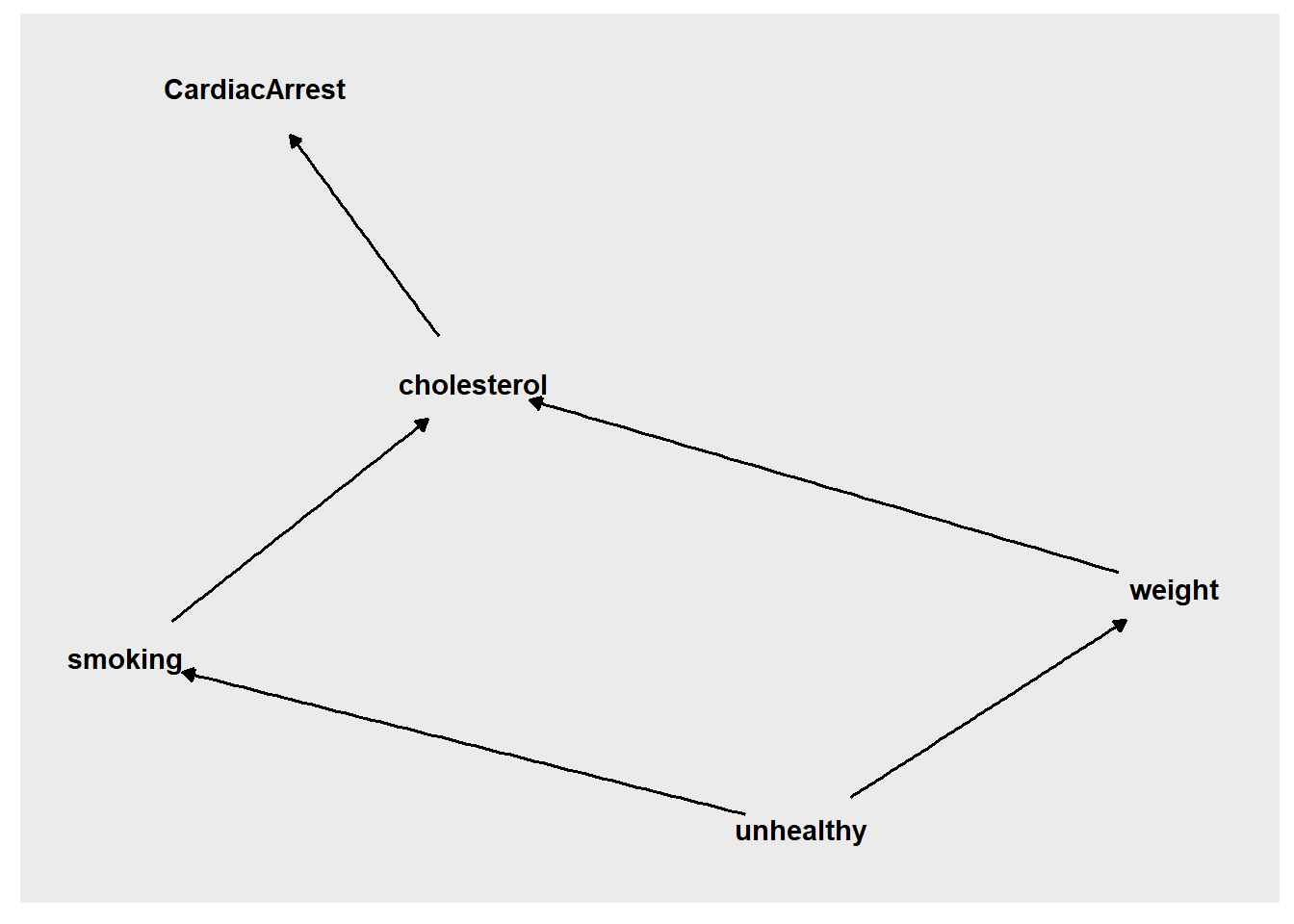

Task 20: In DAG #1, above, where CardiacArrest is our outcome of interest, which variables are colliders?

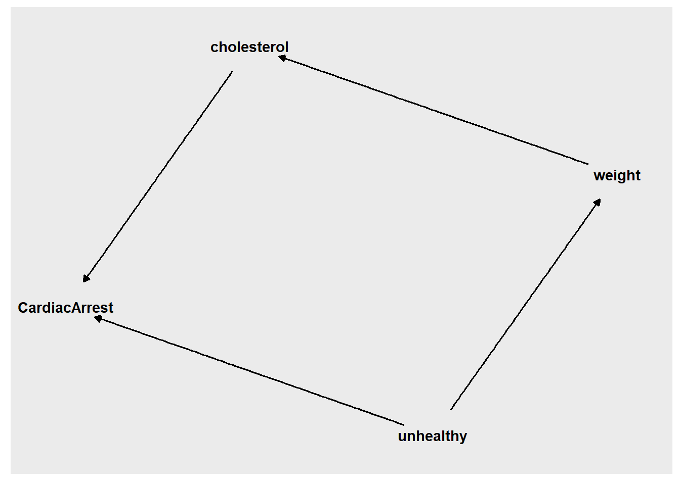
Task 21: In DAG #2, above, if we are interested in the effect of weight on CardiacArrest, does a backdoor path exist between weight and CardiacArrest? If so, what should we do about it, if anything?

Task 22: In DAG #2, if we are interested in the effect of weight on CardiacArrest, which variables are mediators?

Now we will further explore omitted variable bias. Let’s say we are interested in the effect of education (educ) on vocabulary (vocab) score:

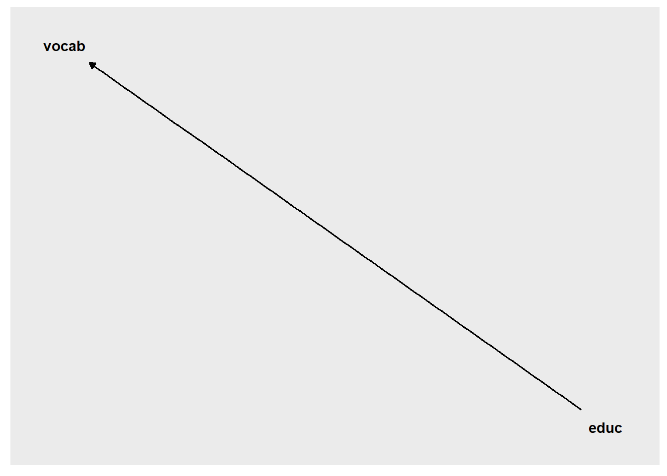
So we run a regression to test this using the GSSvocab dataset, below. Please also run this on your computer using this same code.

if (!require(dplyr)) install.packages('dplyr')
library(dplyr)
if (!require(car)) install.packages('car')
library(car)

v <- GSSvocab %>%
  dplyr::select(vocab, age, educ)
v <- na.omit(v)

reg2 <- lm(vocab~educ,data=v)

summary(reg2)

## 
## Call:
## lm(formula = vocab ~ educ, data = v)
## 
## Residuals:
##     Min      1Q  Median      3Q     Max 
## -8.2851 -1.2770  0.0529  1.3849  8.3950 
## 
## Coefficients:
##             Estimate Std. Error t value Pr(>|t|)    
## (Intercept) 1.604953   0.050086   32.04   <2e-16 ***
## educ        0.334007   0.003711   90.01   <2e-16 ***
## ---
## Signif. codes:  0 '***' 0.001 '**' 0.01 '*' 0.05 '.' 0.1 ' ' 1
## 
## Residual standard error: 1.849 on 27406 degrees of freedom
## Multiple R-squared:  0.2282, Adjusted R-squared:  0.2281 
## F-statistic:  8101 on 1 and 27406 DF,  p-value: < 2.2e-16

You can also run the regression model above on your own computer.

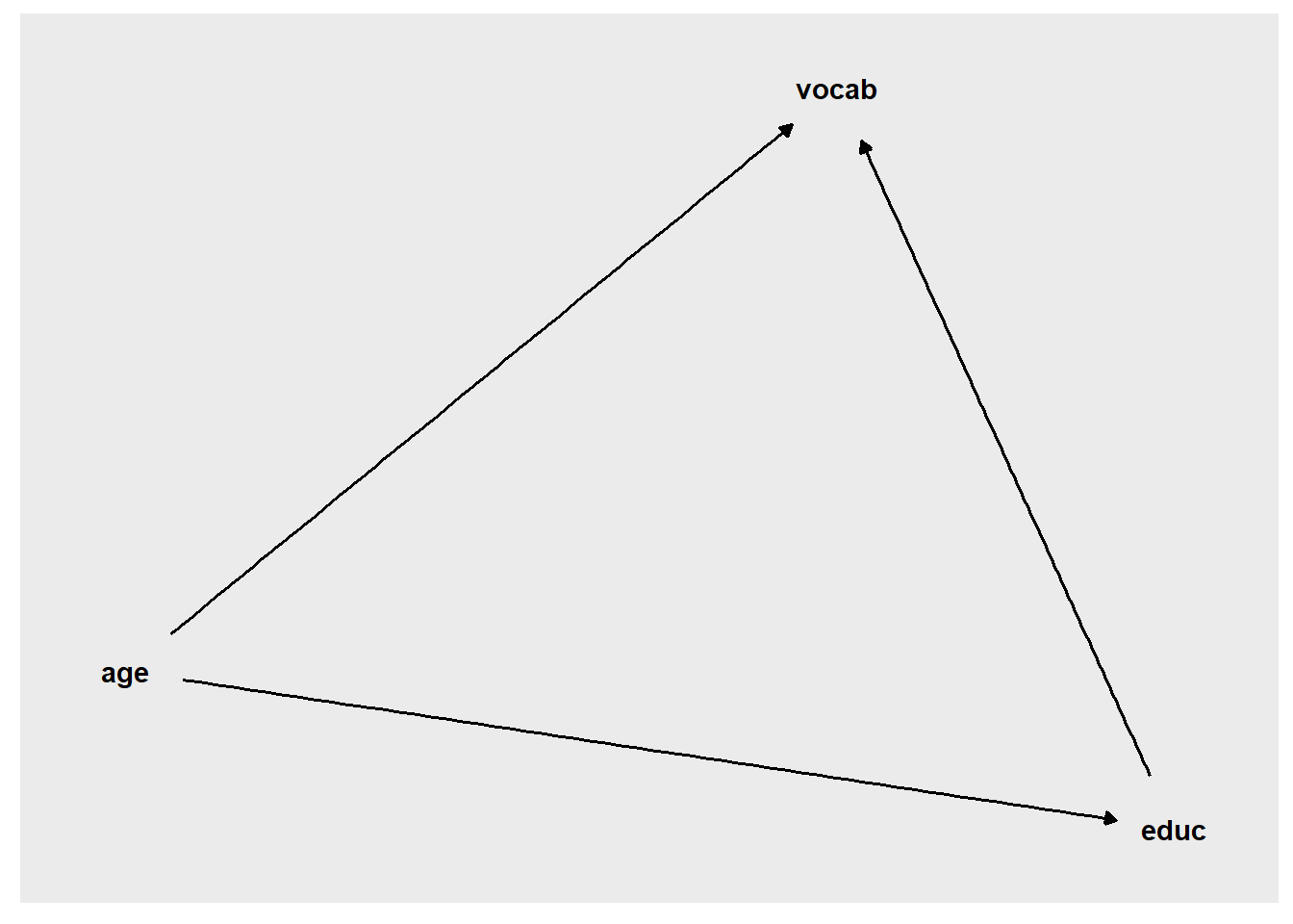
Now we are concerned that age (age), a variable we left out of the regression model, might be an omitted confounding variable, causing our regression estimate to be biased (meaning inaccurate). The following DAG shows this situation:

We can also make the following correlation matrix, which can be used to determine how the omitted variable is associated with the other variables that are involved:

cor(v[c("vocab","age","educ")])

##            vocab         age       educ
## vocab 1.00000000  0.05501119  0.4776605
## age   0.05501119  1.00000000 -0.1312746
## educ  0.47766049 -0.13127456  1.0000000

Task 23: According to the regression model above—with only educ as the independent variable—what is the estimated effect of education on vocabulary? Please answer this question without taking into account any omitted variable bias. This is just to establish what the relationship between education and vocabulary is before we account for omitted variable bias or change the regression model in any way.

Task 24: Write out the equation for the regression output above, including the error term (it will be the equation for \(vocab\) rather than \(\hat{vocab}\)). In the error term, include the term for the omitted variable, using whichever notation you would like (it does not need to be formal).

Task 25: Determine if the education estimate is biased due to omitted variable bias. If the education estimate is biased, in what direction is it biased? Is the true association between education and vocabulary score higher or lower than the equation suggests? Please show your work. Remember that you can refer to the correlation matrix above to learn how the omitted variable is associated with the other variables involved. You do not need to find the exact size of any potential bias, just the direction.

Task 26: Run another regression model to see if there was omitted variable bias and in what direction. What is the new estimated effect of education on vocabulary, now that you have accounted for the omitted variable bias?

8.5.5 Final project brainstorming

As part of this course, you will have to complete a final project. This project will require you to pick a dataset that already exists (which can be one that you already have and plan to do research upon, one that you find specifically for the purposes of this project, or one that course instructors provide for you upon your request), identify a research question that you can investigate using that data, and conduct a statistical analysis to answer the question. You will need to provide a brief write-up of your work, as if you are writing only the methods section and results section of a short academic research paper.

This portion of this assignment is meant to help you prepare for this project.

Task 27: Please click here to read about the final project, if you have not done so already.

Task 28: What data do you want to use for your project? If you have data of your own, explain the data that you have in 3–6 sentences. Make sure you describe the key variables in the data and mention how many observations are in the data (you can include a standardize dataset description of your data, the way we have done in some of our previous assignments). If you do not have data of your own, brainstorm about what data you could use or let the instructors know in your response that you would like us to provide a dataset for you.

Task 29: What research question would you investigate using the data you specified above? If you do not yet have a dataset selected, you do not need to answer this question (and we should meet to discuss which data you could use).

Task 30: What is your hypothesis about the answer to the research question above? If you do not have a research question yet, brainstorm about the types of questions you might be interested in asking, so that we can then think about which already-existing data would be appropriate for your project.

8.5.6 Additional items

You have now reached the end of this week’s assignment. The tasks below will guide you through submission of the assignment, remind you of any other items you need to complete this week, and allow us to gather questions and/or feedback from you.

Task 31: You are required to complete 15 quiz question flashcards in the Adaptive Learner App by the end of this week.

Task 32: Please write any questions you have for the course instructors (optional).

Task 33: Please write any feedback you have about the instructional materials (optional).

Task 34: Knit (export) your RMarkdown file into a format of your choosing.

Task 35: Please submit your assignment to the D2L assignment drop-box corresponding to this chapter and week of the course. And remember that if you have trouble getting your RMarkdown file to knit, you can submit your RMarkdown file itself. You can also submit an additional file(s) if needed.

---

165. Unless your data spreadsheet containing your sample includes all members of your population of interest.↩︎

166. Munroe, Randall. “Correlation.” xkcd: a webcomic of romance, sarcasm, math, and language. https://xkcd.com/552/.↩︎

167. You can also condition on variables through study design. For example, you can condition on gender by restricting your study to only females.↩︎

168. Alternate link, if the main one doesn’t work: https://docplayer.net/8230063-Mgmt-469-model-specification-choosing-the-right-variables-for-the-right-hand-side.html↩︎

169. Alternate link, if the main one doesn’t work: https://docplayer.net/8230063-Mgmt-469-model-specification-choosing-the-right-variables-for-the-right-hand-side.html↩︎

170. In this scenario, you are not interested in training teams, just individuals.↩︎

171. You must have intervention and control groups of 50 people each, you must test an intervention, and you must use the 0–10 point scale as the main measure of the outcome of interest.↩︎