Chapter 5 Multiple OLS Linear Regression and OLS Diagnostic Tests

This week, our goals are to…

Run OLS linear regression with more than one independent variable and interpret the results.
Evaluate OLS regression results to see if they are trustworthy, by running and interpreting diagnostic tests of the OLS assumptions.
Create dummy variables for constructs (variables, for our purposes) with more than two levels.
Use dummy variables in a regression analysis. Interpret and visualize the results.

Announcements and reminders

You might remember that in Chapter 1, there is a section about selected terminology. Previously, many of those terms may not have had meaning to you. Now, most of them should. I recommend that you review that section at some point this week.
You may have noticed on our course calendar that Oral Exam #1 is coming up soon. Each of you will have to schedule an individual meeting time with an instructor for us to do your Oral Exam #1. The calendar shows recommended weeks to do the exam, although doing it later is also acceptable. You have a two-week window to ideally do Oral Exam #1. More information about Oral Exam #1 can be found by clicking here. Please e-mail both Anshul and Nicole with times when you could do your Oral Exam #1.

5.1 Multiple OLS linear regression

Previously, we looked at simple OLS (ordinary least squares) linear regression. In simple OLS, we had one independent variable that we were using to try to predict the values of the dependent variable. To accomplish this, we created a regression model which could be described by an equation. Plugging numbers into the equation gave us predicted values of the dependent variable. We also generated inferential statistics to determine if the relationship between the dependent and independent variable in our sample is also likely the case or not in the population of interest. Finally, we looked at the $R^2$ statistic to determine the goodness-of-fit of our regression model.

In this section, we will replicate the simple OLS process, this time with multiple independent variables that are working together to try to predict the dependent variable. Many of the features that we saw in simple OLS will again be involved with multiple OLS. First let’s clearly distinguish between simple OLS and multiple OLS, below.

Simple compared to multiple OLS linear regression:

Simple OLS linear regression: One independent variable predicting one dependent variable. The dependent variable is the outcome of interest that we care about.
Multiple OLS linear regression: Multiple independent variables predicting one dependent variable. The dependent variable is the outcome of interest that we care about.

Remember:

All regression models have just one dependent variable (outcome of interest). The dependent variable is typically the result or outcome you are interested in, such as how much weight someone can lift, how much somebody’s blood pressure changes, or how well a student does on a test. Independent variables are measurable constructs that we hypothesize are causing or are associated with the dependent variable.
In all cases—simple linear regression, multiple linear regression, or other types of regression we will learn later—all regression analyses are using numbers to help us answer a question. We will always start with a question we want to answer, define relevant metrics (variables, for our purposes), make sure all aspects of our research design are responsible and logical, and then run a regression analysis to try to answer the question. Then we evaluate how well-fitting and trustworthy our results are before drawing a final conclusion (an answer to our question). This procedure is universal, even when the specific regression methods change.

In the rest of this section, we will learn how to run a multiple OLS linear regression, interpret its results, and evaluate its goodness-of-fit.

5.1.1 Multiple OLS linear regression in R

In this section, we will run a multiple OLS linear regression model in R and interpret the results. We will continue to use the mtcars dataset that was used earlier in this textbook to introduce simple OLS. Note that “multiple” OLS regression refers to a regression analysis in which there is more than one independent variable, which is the focus of this section. It is fine to refer to a regression model with multiple independent variables as a multiple OLS linear regression, multiple linear regression, OLS linear regression, or linear regression. All of these terms mean the same thing. The terms regression analysis and regression model can also be used interchangeably. They mean the same thing, for our purposes.

Here are the key details of the example regression analysis we will conduct:

Question: What is the association between displacement and weight in cars, controlling for rear axle ratio and transmission?⁸⁶
Dependent variable: disp; displacement in cubic inches.
Independent variables: wt, weight in tons; drat, rear axle ratio; and am, transmission type.
Dataset: mtcars data in R, loaded as d in our example.

Run the following code to load the data and follow along with the example:

d <- mtcars

Note that you can also run the following code to learn more about this data:

?mtcars

Remember that d is a copy of the dataset mtcars. We will do all of our analysis on the dataset d.

Keep reading to see how we can try to answer our question above using multiple OLS regression!

5.1.2 Examine variables before running regression

Before we run a multiple linear regression, it can help to inspect our data first in a variety of ways. We have already learned how to calculate descriptive statistics for individual variables, make one-way and two-way tables, and make grouped descriptive statistics. Another useful way to learn about your data is to make a correlation matrix.

The code below creates a fancy correlation matrix for us:

if (!require(PerformanceAnalytics)) install.packages('PerformanceAnalytics')
library(PerformanceAnalytics)

chart.Correlation(d, histogram = TRUE)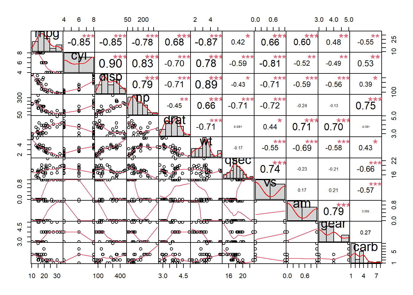

With the code above, here is what we asked the computer to do for us:

if (!require(PerformanceAnalytics)) install.packages('PerformanceAnalytics') – Check if the PerformanceAnalytics package is already installed and install it if not.
library(PerformanceAnalytics) – Load the PerformanceAnalytics package.
chart.Correlation(d, histogram = TRUE) – Run the function chart.Correlation(...), which creates a correlation matrix. We put two arguments in the chart.Correlation(...) function: d tells the computer that we want a correlation matrix of the variables in the dataset d. histogram = TRUE tells the computer that we also want it to include a histogram of the distribution of each variable along the diagonal of the correlation matrix.

Let’s interpret the correlation matrix that we got, focusing on the following key items:

The matrix shows us the pairwise relationships—meaning each combination of two variables separately—for all variables in our dataset d.
On the diagonal from the top-left to bottom-right we see the name of each variable and a histogram of how that variable is distributed. For example, we see that the variable disp might be bimodal. We see that the variable am has just two possible values.
In the top-right half of the matrix, we see the numeric correlation coefficients calculated for each pair of variables. For example, we see that disp and drat are correlated at -0.71. disp and wt are correlated at 0.89.
In the bottom-left half of the matrix, we see scatterplots of each combination of variables. This tells us, for example, that disp and hp appear to be highly correlated, while wt and qsec are not highly correlated.

You may have noticed that the correlation matrix above is pretty large and hard to read. It also involves many variables that are unrelated to us answering our question of interest. Let’s make a smaller matrix that is more specific to our current goals.

The code below creates a copy of the dataset d called d.partial⁸⁷ which only contains the four variables that we are going to use:

d.partial <- mtcars[c("disp","wt","drat", "am")]

And now we can recreate the correlation matrix only for d.partial:

if (!require(PerformanceAnalytics)) install.packages('PerformanceAnalytics')
library(PerformanceAnalytics)

chart.Correlation(d.partial, histogram = TRUE)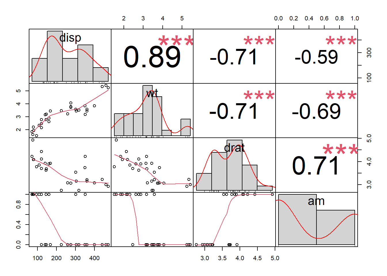

Above, we see an easier-to-read correlation matrix with only our variables of interest. Note that it was NOT necessary to make the first, larger matrix before we made the second, more readable one. We can go straight to the second one without making the first one.

We will not necessarily always make a correlation matrix if we are doing an analysis with a large number of variables, but it is good to look at some pairwise correlations if possible before you continue with your analysis.

5.1.3 Multiple OLS in our sample

Let’s start to answer our question articulated above by making a multiple OLS linear regression model. Remember, our question of interest is: What is the association between displacement and weight in cars, controlling for rear axle ratio and transmission?

The code below runs a multiple OLS regression to address our question within our sample of 32 observations:

reg1 <- lm(disp~wt+drat+am, data = d)

Here is what we are telling the computer to do with the code above:

reg1 – Create a new regression object called reg1. This can be named anything, not necessarily reg1.
<- – Assign reg1 to be the result of the output of the function lm(...)
lm(...) – Run a linear model using OLS linear regression.
disp – This is the dependent variable in the regression model.
~ – This is part of a formula. This is like the equals sign within an equation.
wt – This is the first independent variable in the regression model.
+ – This is a plus sign. We put a plus sign in between all independent variables in the regression model we are making.
drat – This is the second independent variable in the regression model.
am – This is the third independent variable in the regression model. We can add an unlimited number of independent variables. In this case we stopped at three.
data = d – Use the dataset d for this regression. d is where the dependent and independent variables are located. If our dataset had a different name, like mydata or aldfji, then we would replace d with mydata or aldfji in this part of the code.

Note that the independent variables can be listed after the ~ in any order (separated by + signs, of course). You can try changing the order and you will see that you get the same results each time!

If you look in the Environment tab in RStudio, you will see that reg1 is saved and listed there. Our regression results are stored as the object reg1 in R and we can refer back to them any time we want, as we will be doing multiple times below.

We are now ready to inspect the results of our regression model by using the summary(...) function to give us a summary of reg1, like this:

summary(reg1)

## 
## Call:
## lm(formula = disp ~ wt + drat + am, data = d)
## 
## Residuals:
##    Min     1Q Median     3Q    Max 
## -62.52 -44.03 -13.08  28.12 136.55 
## 
## Coefficients:
##             Estimate Std. Error t value Pr(>|t|)    
## (Intercept)    62.14     137.78   0.451    0.655    
## wt            104.81      16.09   6.512 4.67e-07 ***
## drat          -50.75      30.29  -1.675    0.105    
## am             34.23      31.57   1.084    0.288    
## ---
## Signif. codes:  0 '***' 0.001 '**' 0.01 '*' 0.05 '.' 0.1 ' ' 1
## 
## Residual standard error: 57.03 on 28 degrees of freedom
## Multiple R-squared:  0.8088, Adjusted R-squared:  0.7883 
## F-statistic: 39.47 on 3 and 28 DF,  p-value: 3.438e-10

Above, we see summary output of our regression model. The most important section that we will look at first is the Coefficients section of the output. We will use these coefficients to write the equation of our regression model.

Here are some new details about multiple regression model equations:

So far in this textbook, we have written a simple regression equation like this: $\hat{y}=b_1x+b_0$
Now we will write a more complicated multiple regression equation like this: $\hat{y}=b_1x_1+b_2x_2+...+b_0$.
- There will now be one $x_{something}$ for each independent variable in our regression model.
- There will now be one $b_{something}$ number for each predicted slope in our regression model. $b_1, b_2, b_3$ and so on (one for each independent variable) can be called the slopes, coefficients, or betas of the regression model. It is fine to write these as $b$, $B$, or $\beta$.
- There will still be a single $b_0$ which represents the intercept of the regression model. This still tells us the predicted value of the dependent variable when the values of all independent variables are 0.
- There is still a $\hat{y}$ on the left side of the equation, representing the predicted value(s) of the single dependent variable that is our outcome of interest.

Here is the regression equation for reg1: $\hat{disp} = 104.81 wt - 50.75 drat + 34.23 am + 62.14$

This equation came directly from the regression table:

104.81 is the coefficient of wt in the summary table. This means that in our sample, for every one ton increase in wt, disp is predicted to increase by 104.81 cubic inches on average, controlling for the other independent variables drat and am.
-50.75 is the coefficient of drat in the summary table. This means that in our sample, for every one unit increase in drat, disp is predicted to decrease by 50.75 cubic inches on average, controlling for the other independent variables wt and am.
34.23 is the coefficient of am in the summary table. am is a dummy variable. The computer doesn’t “know” this (the computer just thinks that am is a continuous numeric variable like the others), but we do.
- If am had been a typical continuous numeric variable, here is how we would interpret its coefficient: In our sample, for every one unit increase in am, disp is predicted to increase by 34.23 cubic inches on average, controlling for the other independent variables wt and drat.
- However, since am is a dummy variable, we humans can interpret it differently. Note that observations that have am coded as 0 are cars with an automatic transmission. And observations with am coded as 1 are cars with a manual transmission. For us humans, a “one-unit increase in am” can only possibly represent a change from 0 to 1. A change from 0 to 1 in am means a change from automatic (which is 0) to manual (which is 1).
- This is how we humans interpret the am coefficient: In our sample, a car with manual transmission is predicted to have a value of disp that is on average 34.23 cubic inches higher than the disp of a car with automatic transmission, controlling for wt and drat.
- Here’s another way to think about it: the dummy variable am divides our 32 observations into two groups, those with automatic transmission (am = 0) and those with manual transmission (am = 1). When we put the dummy variable am into the regression, the result just tells us the estimated average difference in the dependent variable disp between automatic and manual cars. Dummy variables just help us estimate differences between two groups.

Notice the following characteristics of our results and interpretation of our regression results for our sample:

In our interpretation of the regression results, we always used the words predicted and average. This is because the relationship between the dependent variable disp and any of the independent variables is not a true exact relationship. It is a best guess about the relationship. This best guess is just an average trend across all of the observations in our sample. It is not the exact truth that if we added one ton of weight to a car, its disp would increase by exactly 104.81 cubic inches. Instead, 104.81 cubic inches is just the predicted average increase in disp for each additional ton heavier a car is.
All of the relationships that we calculated in our regression results are associations, not causal relationships. We did NOT find that each one unit increase in drat causes an average decrease of 50.75 cubic inches in disp. We merely found that each one unit increase in drat is associated with an average decrease of 50.75 cubic inches in disp, when controlling for wt and am.
The key part of our interpretations of the slopes in our regression results were the magic words “For every one unit increase in X…,” with “X” referring to any of the independent variables. These are the first words that should come to your mind when you try to interpret a regression result. It may be worthwhile to write these words on a sticky note next to your workstation until you have them memorized.
The question we initially wanted to answer only concerned the relationship between the dependent variable disp and the independent variable wt. drat and am were just supposed to be control variables that we adjusted for in the regression model. But why did we interpret the results above without giving any special attention to the wt coefficient? Well, from the computer’s perspective, it is calculating for us the relationship between the dependent variable and each independent variable one at a time, controlling for any other independent variables. So this regression model is actually answering three questions all at once, even though we only care about the answer to the first one:
- What is the relationship between disp and wt, controlling for drat and am?
- What is the relationship between disp and drat, controlling for wt and am?
- What is the relationship between disp and am, controlling for wt and drat?
It is important to note that any relationships we found between variables are just associations rather than causal relationships.

With our regression equation—$\hat{disp} = 104.81 wt - 50.75 drat + 34.23 am + 62.14$—we can calculate predicted values for our dependent variable disp by plugging in values of wt, drat, and am.

Let’s practice calculating a predicted value of disp for an observation (a car, in this case) with the following characteristics:

Name of car: Yalfo
wt = 2 tons
drat = 2 units
manual transmission

We follow these steps to make the prediction:

Start with initial regression equation: $\hat{disp} = 104.81 wt - 50.75 drat + 34.23 am + 62.14$
Slightly re-write initial regression equation, for clarity: $\hat{disp} = (104.81*wt) + (-50.75*drat) + (34.23*am) + 62.14$
Plug specific characteristics of Yalfo into equation: $\hat{disp} = (104.81*2) + (-50.75*2) + (34.23*1) + 62.14 = 204.49 \text{ cubic inches}$

Note that we plugged in 1 for am since Yalfo has a manual transmission and am is coded as 1 for observations with manual transmissions.

R can do the calculation for us with the following code:

(104.81*2) + (-50.75*2) + (34.23*1) + 62.14

## [1] 204.49

You can put the code above into an R code chunk in RMarkdown and run it to get the answer (which in this case is our predicted value for Yalfo).

Now let’s imagine another car called the Yalfo-2. Yalfo-2 is the same as Yalfo except Yalfo-2 has an automatic transmission. Then we would change am from 1 (for the manual Yalfo) to 0 (for the automatic Yalfo-2), like this:

\[\hat{disp} = (104.81*2) + (-50.75*2) + (34.23*0) + 62.14 = 170.26 \text{ cubic inches}\]

The Yalfo has a predicted displacement of 204.49 cubic inches and the Yalfo-2 has a predicted displacement of 170.26 cubic inches. This is a difference of $204.49 - 170.26 = 34.23 \text{ cubic inches}$. This difference is the same value as the coefficient of am! We just demonstrated that the coefficient of the dummy variable am tells us the predicted difference between a car with manual transmission and automatic transmission.

Let’s practice one more important calculation of a predicted value of another hypothetical observation (another car):

Name of car: FeatherMobile
wt = 0 tons
drat = 0 units
automatic transmission

We plug the characteristics of the FeatherMobile into the regression equation:

\[\hat{disp} = (104.81*0) + (-50.75*0) + (34.23*0) + 62.14 = 62.14 \text{ cubic inches}\]

This shows that the intercept of a regression model is the predicted value of the dependent variable—disp, in this case—when all of the independent variables are 0. As we discussed when we learned about simple regression, the intercept is often meaningless. In this case, there is no such thing as a car that is weightless, so the intercept is meaningless. Nevertheless, it is important to know what the intercept theoretically represents.

Our regression model tells us the exact predicted relationship on average between displacement and weight in our sample. Everything written above has pertained to our sample only. We will now turn our attention to inference and our population of interest.

5.1.4 Multiple OLS in our population

We are now interested in answering this question: What is the true relationship between disp and wt in the population from which our sample was selected, when controlling for drat and am?

To answer this question, we have to look at some of the inferential statistics that are calculated when we do a regression analysis. We also need to conduct some diagnostic tests of assumptions before we can trust the results.

We will start by calculating the 95% confidence intervals for our estimated regression coefficients, by running the confint(...) function on our saved regression results—called reg1—like this:

confint(reg1)

##                  2.5 %    97.5 %
## (Intercept) -220.08792 344.36793
## wt            71.84099 137.77595
## drat        -112.79506  11.29956
## am           -30.44439  98.89628

It is also possible to create a regression summary table that contains everything we need all in one place, using the summ(...) function from the jtools package.

Run the following code to load the package and see our regression results:

if (!require(jtools)) install.packages('jtools')
library(jtools)

summ(reg1, confint = TRUE)

Observations	32
Dependent variable	disp
Type	OLS linear regression

F(3,28)	39.47
R²	0.81
Adj. R²	0.79

	Est.	2.5%	97.5%	t val.	p
(Intercept)	62.14	-220.09	344.37	0.45	0.66
wt	104.81	71.84	137.78	6.51	0.00
drat	-50.75	-112.80	11.30	-1.68	0.10
am	34.23	-30.44	98.90	1.08	0.29
Standard errors: OLS

Here is what the lines of code above accomplished:

if (!require(jtools)) install.packages('jtools') – Check if the jtools package is already installed and install it if not.
library(jtools) – Load the jtools package.
summ(reg1, confint = TRUE) – Create a summary output of the saved reg1 regression result. Include the confidence intervals (because confint is set to TRUE).

We can now interpret the 95% confidence intervals that were calculated:

wt: In the population from which our sample was drawn, we are 95% confident that the slope of the relationship between displacement and weight is between 71.84 and 137.78 cubic inches, controlling for drat and am. In other words: In our population of interest, we are 95% confident that for every one ton increase in a car’s weight, its displacement is predicted to increase by at least 71.84 cubic inches or at most 137.78 cubic inches, controlling for drat and am. Since this 95% confidence interval is entirely on one side of 0—above, in this case—we can conclude with high certainty that there is a positive relationship in the population between disp and wt. This is the answer to our question of interest, if our data passes all diagnostic tests that we will conduct later.
drat: In the population from which our sample was drawn, we are 95% confident that the slope of the relationship between displacement and rear axle ratio is between -112.80 and 11.30 cubic inches, controlling for wt and am. In other words: In our population of interest, we are 95% confident that for every one unit increase in a car’s rear axle ratio, its displacement is predicted to change by at least -112.80 cubic inches or at most 11.30 cubic inches, controlling for drat and am. Since this 95% confidence interval includes 0, we cannot conclude that there is a non-zero relationship of any kind between disp and drat. The true relationship could be negative, zero, or positive. We didn’t find any definitive evidence. Note that even though we did not find a definitive answer about the relationship between disp and drat, we still did successfully control for the variable drat. The findings from this regression model about the relationships between a) disp and wt and b) disp and am are still legitimate.
am: In the population from which our sample was drawn, we are 95% confident that manual transmission cars have displacements that are between 30.44 cubic inches lower⁸⁸ and 98.90 cubic inches higher than automatic transmission cars, controlling for weight and rear axle ratio. Since this confidence interval crosses 0, we did not find evidence of a non-zero relationship between disp and am. We did, however, successfully control for am in this regression, such that we might be able to draw conclusive answers about the relationship between the dependent variable disp and other independent variables wt and drat.
Intercept: In the population from which our sample was drawn, we are 95% confident that a car that weighs 0 tons, has a rear axle ratio of 0 units, and has automatic transmission has a displacement that is between -220.09 and 344.37 cubic inches. We are again not at all confident about what this predicted value might truly be in the population, and that is okay.

Like with simple regression, the computer conducted a number of hypothesis tests for us when it ran our regression analysis. For example, one of these hypothesis tests relates to the slope estimate for displacement and weight.

Here is the framework for this hypothesis test:

$H_0$: In the population of interest, $b_{wt} = 0$. In other words: in the population of interest, there is no relationship between displacement and weight of cars.
$H_A$: In the population of interest, $b_{wt} \ne 0$. In other words: in the population of interest, there is a non-zero relationship between displacement and weight of cars.

The result of this hypothesis test is within the regression output. The p-value for weight is extremely small. This means that we have very high confidence in the alternate hypothesis $H_A$, meaning that there likely is an association between displacement and weight in our population of interest. More specifically, we are 95% confident that the slope of the association between displacement and weight in the population is between 71.84 and 137.78 cubic inches. Taking the p-value and confidence intervals into consideration, we reject the null hypothesis (if our diagnostic tests of OLS assumptions go well, later).

Here are some important reminders about our multiple OLS linear regression results:

All of the estimated coefficients are measured in units of the dependent variable.
The slope of 104.81 cubic inches is the true average relationship between displacement and weight in our sample alone.
The 95% confidence intervals and p-values pertain to the population.
The slope of 104.81 cubic inches is the midpoint of the 95% confidence interval.
None of these results for the population of interest can be trusted until certain diagnostic tests of assumptions have been conducted.
It is important to note that any relationships we found between variables are just associations rather than causal relationships.

5.1.5 Graphing multiple OLS results

With simple linear regression, it was easy to graph our regression results because we just had two variables—our dependent variable and one independent variable—to graph and a scatterplot has two dimensions. But now with multiple regression, we have four variables—our dependent variables and three independent variables. So how can we visualize our results?

There are many possibilities. We will learn just one in this section. Since our primary relationship of interest is between disp and wt, let’s make our scatterplot have disp on the vertical axis (because that’s always where we put the dependent variable) and wt on the horizontal axis. Then, since am is a dummy variable, we can draw two separate lines showing predicted values for observations that fall into each group of am.

This code plots disp against wt along with the two prediction lines:⁸⁹

if (!require(interactions)) install.packages('interactions')
library(interactions)

interact_plot(reg1, pred = wt, modx = am, plot.points = TRUE)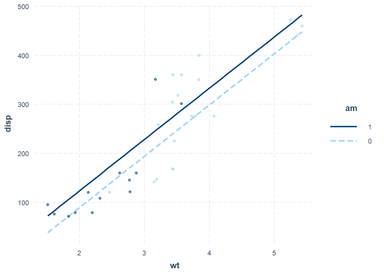

In the code we used to generate this scatterplot, here is what we asked the computer to do:

First we installed (if necessary) and loaded the interactions package.
interact_plot(reg1, pred = wt, modx = am, plot.points = TRUE) – Create a scatterplot using the interact_plot(...) function. The interact_plot(...) function has four arguments:
- reg1 – We will be making a scatterplot based on the regression model reg1.
- pred = wt – We want the predictor (meaning independent variable) on the horizontal axis to be wt. Note that the vertical axis will be our dependent variable disp by default; we don’t need to tell the computer that.
- modx = am – Here we specify that am is the moderator variable out of all the independent variables. This tells the computer to draw separate regression lines for predictions in each category of am.
- plot.points = TRUE – Plot individual data points on the scatterplot, in addition to showing regression lines.

Now we can turn to interpreting the scatterplot:

Dark blue points show the true (actual) disp and wt of cars with manual transmissions in our data.
The dark blue line shows the predicted relationship between disp and wt calculated by our regression model for cars with manual transmissions.
Light blue points show the true (actual) disp and wt of cars with automatic transmissions in our data.
The light blue line shows the predicted relationship between disp and wt calculated by our regression model for cars with automatic transmissions.
Remember that our regression model predicts that in our sample, cars with manual transmissions will have a disp that is 34.23 cubic inches higher than cars with automatic transmissions, controlling for the other two independent variables. This predicted difference of 34.23 cubic inches between these two types of cars is shown visually in the scatterplot. Choose any weight and check this for yourself. Let’s consider a car that weighs 3 tons. If this 3-ton car has automatic transmission, its predicted disp is around 190 cubic inches on the scatterplot. If this 3-ton car has manual transmission, its predicted disp is around 225 cubic inches on the scatterplot. This is a difference of about 35 cubic inches, which is almost the same value as our coefficient of am which is 34.23 cubic inches!
We see that when we controlled for wt, meaning we looked at just a single value of wt, the difference between am = 1 observations and am = 0 observations is around 34.23 cubic inches. If we looked at a different value of wt, such as 4.5 tons, the difference between automatic and manual cars would still be 34.23 cubic inches. This is what it means to control for one independent variable—wt, in this case—while looking at the relationship between the dependent variable (disp) and another independent variable am.
The scatterplot also shows that our regression model successfully controlled for am when considering the relationship between disp and wt. We know this because the two lines in the plot are parallel. The slope defining the relationship between disp and wt is the same regardless of which line you choose to look at. This is what it means to control for am. We uncovered the relationship between the dependent variable disp and another independent variable wt regardless of the value of am.
Another useful way to think about a dummy variable is that it shifts the intercept of a regression model for a particular group. Let’s see how this is the case:
- Start with the regression equation from our regression model reg1: $\hat{disp} = 104.81 wt - 50.75 drat + 34.23 am + 62.14$.
- Plug in am = 0 for observations (cars) with automatic transmission: $\hat{disp} = 104.81 wt - 50.75 drat + 34.23*0 + 62.14$. We then simplify this into a final regression equation only for cars with automatic transmission: $\hat{disp}_\text{automatic transmission} = 104.81 wt - 50.75 drat + 62.14$.
- Plug in am = 1 for observations (cars) with manual transmission: $\hat{disp} = 104.81 wt - 50.75 drat + 34.23*1 + 62.14$. We then simplify this into a final regression equation only for cars with manual transmission: $\hat{disp}_\text{manual transmission} = 104.81 wt - 50.75 drat + 96.37$.
- Notice above that we created two equations—one for $\hat{disp}_\text{automatic transmission}$ and another for $\hat{disp}_\text{manual transmission}$. Once we simplified these equations, they are exactly the same except they have different intercepts.
The scatterplot also give us a visual sense for how well our regression model fits our data. The closer the plotted points are to the line(s), the better fitting our regression line is.

5.1.6 Generic code for multiple OLS linear regression in R

This section contains a generic version of the code and interpretation that you can use to run a multiple OLS linear regression in R. You can copy the code below and follow the guidelines to replace elements of this code such that it is useful for analyzing your own data.

To run an OLS linear regression in R, you will use the lm(...) command:

reg1 <- lm(DepVar ~ IndVar1 + IndVar2 + IndVar3 + IndVar4 + ..., data = mydata)

Here is what we are telling the computer to do with the code above:

reg1 – Create a new regression object called reg1. You can call this whatever you want. It doesn’t need to be called reg1.
<- – Assign reg1 to be the result of the output of the function lm(...)
lm(...) – Run a linear model using OLS linear regression.
DepVar – This is the dependent variable in the regression model. You will write the name of your own dependent variable instead of DepVar.
~ – This is part of a formula. This is like the equals sign within an equation. The ~ goes after the dependent variable and before the independent variables.
IndVar1 – This is the first independent variable in the regression model. You will write the name of one of your own independent variables here instead of IndVar.
+ – This is a plus sign. All of your independent variables should be listed, separated by plus signs.
IndVar2–IndVar4 – These are additional independent variables. You will write the names of the variables from your own dataset in place of these. You can have as many or as few independent variables as you would like. The order in which you input the independent variables doesn’t matter, as long as they are all after the ~, separated by plus signs, and before the comma.
data = mydata – Use the dataset mydata for this regression. mydata is where the dependent and independent variables are located. You will replace mydata with the name of your own dataset.

Then we would run the following command to see the results of our saved regression, reg1:

summary(reg1)

The summary(...) function shows you the results of the regression that you created and saved as reg1.

If you look in your Environment tab in RStudio, you will see that reg1 (or whatever you called your regression) is saved and listed there.

A summary table with confidence intervals can be created with the following code:

if (!require(jtools)) install.packages('jtools')
library(jtools)

summ(reg1, confint = TRUE)

5.2 Residuals in multiple OLS

We will continue using the reg1 regression model that we created earlier in this chapter, which examined the relationship between displacement and weight of cars. Earlier in the chapter, our focus was on interpreting the slopes and intercept in the regression model. Now we will turn our attention to an analysis of the individual observations in our dataset. Below, we will examine errors between our actual and predicted values of displacement in our regression model.

Remember: Displacement (disp) is our dependent variable; and weight (wt), rear axle ratio (drat), and transmission type (am) are our independent variables in this regression model. The dependent variable is our outcome of interest that we care about. Just like in simple OLS, our main concern when we analyze residuals and error is our predictions of the dependent variable made by the regression model. Most of the procedure below is based on the dependent variable alone, which is displacement (disp).

Now we are going to calculate the predicted values (also called fitted values) for our regression model reg1. This follows the same process and code that we used for simple OLS previously.

Here we calculate predicted values in R:

d$disp.predicted <- predict(reg1)

Inspect new variable in d called disp.predicted:

View(d)

We run the following code to calculate the regression residuals:

d$disp.resid <- resid(reg1)

Now a new variable called disp.resid has been added to our dataset d. You can inspect this new variable by opening d in R on your own computer, using the View(...) command:

View(d)

In the table below, you can see our independent variable (wt), dependent variable (disp), predicted values of the dependent variable (disp.predicted), and the residuals (disp.resid):

d[c("wt","disp","disp.predicted","disp.resid")]

##                        wt  disp disp.predicted disp.resid
## Mazda RX4           2.620 160.0      173.04790 -13.047902
## Mazda RX4 Wag       2.875 160.0      199.77406 -39.774061
## Datsun 710          2.320 108.0      144.14275 -36.142749
## Hornet 4 Drive      3.215 258.0      242.79615  15.203849
## Hornet Sportabout   3.440 360.0      262.82571  97.174286
## Valiant             3.460 225.0      284.71351 -59.713506
## Duster 360          3.570 360.0      273.40595  86.594051
## Merc 240D           3.190 146.7      209.21981 -62.519811
## Merc 230            3.150 140.8      193.35549 -52.555489
## Merc 280            3.440 167.6      223.74994 -56.149945
## Merc 280C           3.440 167.6      223.74994 -56.149945
## Merc 450SE          4.070 275.8      332.91487 -57.114869
## Merc 450SL          3.730 275.8      297.27999 -21.479990
## Merc 450SLC         3.780 275.8      302.52041 -26.720413
## Cadillac Fleetwood  5.250 472.0      463.69355   8.306454
## Lincoln Continental 5.424 460.0      478.37788 -18.377877
## Chrysler Imperial   5.345 440.0      458.42603 -18.426025
## Fiat 128            2.200  78.7      119.89375 -41.193750
## Honda Civic         1.615  75.7       15.44521  60.254793
## Toyota Corolla      1.835  71.1       74.53397  -3.433974
## Toyota Corona       2.465 120.1      132.72619 -12.626194
## Dodge Challenger    3.520 318.0      291.00201  26.997986
## AMC Javelin         3.435 304.0      262.30167  41.698329
## Camaro Z28          3.840 350.0      275.31540  74.684595
## Pontiac Firebird    3.845 400.0      308.82549  91.174514
## Fiat X1-9           1.935  79.0       92.11951 -13.119506
## Porsche 914-2       2.140 120.3       95.84353  24.456471
## Lotus Europa        1.513  95.1       63.62214  31.477865
## Ford Pantera L      3.170 351.0      214.45328 136.546721
## Ferrari Dino        2.770 145.0      202.97854 -57.978543
## Maserati Bora       3.570 301.0      290.88514  10.114863
## Volvo 142E          2.780 121.0      179.16023 -58.160229

Let’s review everything we just did (this process is exactly the same now with multiple OLS as it was for simple OLS):

Calculate the predicted values of disp for each observation—meaning each car, in this case—in our dataset, by plugging each car’s wt, drat, and am value into the regression equation $\hat{disp} = 104.81 wt - 50.75 drat + 34.23 am + 62.14$. These predicted values appear in the table above in the disp.predicted column.
Calculate the residual error for each observation—still meaning each car—in our dataset by calculating the difference between each car’s actual displacement (disp column) and predicted displacement (disp.predicted column). These residual errors appear in the disp.resid column.
We are now ready to use the residuals to quantify and describe error in our regression model. Remember that we want the residuals (residual errors) to be as small as possible.

5.3 R-squared metric of goodness of fit in multiple OLS

All regression models have a variety of goodness-of-fit measures that help us understand how well the entire regression model fits our data and/or how appropriate it is for our data. In this section, we will learn about the measure called $R^2$. This measure is referred to as “R-squared”, “R-square”, “Multiple R-squared”, or something similar. They all mean the same thing.

You already know how to calculate $R^2$ in simple OLS. The process for calculating $R^2$ in multiple OLS is the same. It is all based on the dependent variable, predicted values of the dependent variable, and the residuals. We will continue to use our reg1 example about cars in this section.

If you look at the summary table that we made for reg1, you will see that $R^2 = 0.81$. This number can also be interpreted as 81%. This means that 81% of the variation in the Y variable disp is accounted for by variation in the X variables wt, drat, and am. This is a very high $R^2$ in the context of social science, behavioral, health, and education data. Every time you run an OLS regression (and many other types of regressions as well), you should examine the $R^2$ statistic to see how well your regression model fits your data.

The $R^2$ statistic tells us how well our independent variable helps us predict the value of our dependent variable. Our ultimate goal is to make good predictions of the dependent variable by fitting the best regression line possible to the data. Once you know the $R^2$ of a regression model, you can also use that to compare it to other regression models to see which model has the better fitting line. We will practice doing this later in this textbook.

Most importantly, keep the following in mind about $R^2$:

If $R^2$ is…	How is the model fit?	The residual errors are…	In a scatterplot with a regression line and plotted points…
high	good	small	The points are close to the line
low	bad	big	The points are far away from the line

As you saw when studying simple OLS, $R^2$ has an interesting connection to correlation. $R^2$ is the square of the correlation of the actual and predicted values in any OLS linear regression. We will demonstrate this by calculating in R, below.

5.3.1 Correlation and R-squared

This procedure is the same as the one we used for simple OLS and is presented below in abbreviated form.

Remember:

The actual values are the true outcome numbers of the dependent variable that truly occurred and were measured in reality on our observations.
The predicted values are the best guesses (predictions) that the independent variables in our regression model are able to make about the actual values of the dependent variable. These predicted values represent the variation in the independent variables that the regression model is using to make the predictions.
The correlation of the actual values (true outcomes) and predicted values (best guesses) tells us how well-fitting our regression model is.

We have already calculated the predicted values from our regression model and added them to our dataset d in a variable called disp.predicted. And of course our actual values are simply the ones held in the disp variable in d. So we are all set to visualize and calculate the correlation of these variables.

We can visualize this correlation in a scatterplot:

plot(d$disp.predicted,d$disp)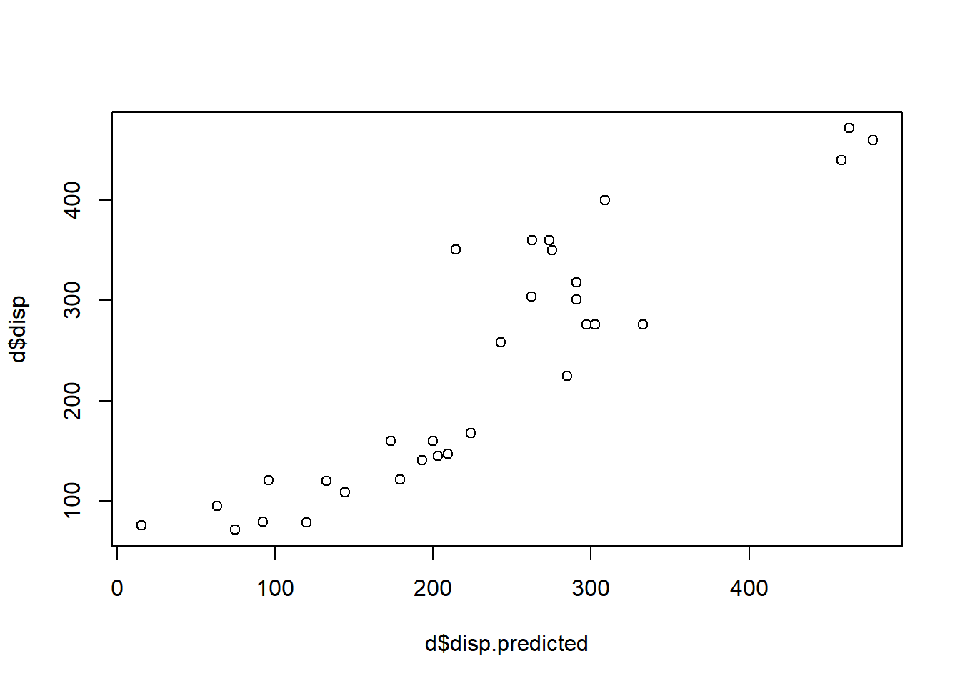

Above, disp.predicted represents ALL of the independent variables (because all of these variables were used to calculate predicted values from the regression equation) and disp is of course our actual values.

The code below calculates the correlation between our actual and predicted values in reg1:

cor(d$disp,d$disp.predicted)

## [1] 0.8993098

Now we save this correlation:

r.reg <- cor(d$disp,d$disp.predicted)

And like before, we square this correlation value:

r.reg^2

## [1] 0.8087581

Once again, we see that the square of the correlation of the actual and predicted values is equal to $R^2$ in our regression model. This is always the case and it is a great way to remember what $R^2$ helps us measure.

Let’s break it down step by step:

The actual values are the true/real outcomes of interest (values of the dependent variable) in our observations (rows of data).
The predicted values are the best guess that we can make about the values of the dependent variable using only the independent variables. That last part is the key. We used only the independent variables to generate the predicted values, by plugging them into the regression equation.
We want to know: How well can the independent variables make predictions of the dependent variable? It turns out that we have everything we need now to answer this question.
We look at the correlation of the predicted values (which represents the best guess made only by the independent variables) with the actual values (which are the true numbers we are trying to predict). This tells us how well the independent variables are able to predict or explain the dependent variable.
We square the correlation that we just calculated so that it is the same as the other way to calculate goodness-of-fit, which is $R^2 = 1 - \frac{SSR}{SST}$, as you know from before.

5.3.2 Calculating R-squared

Now we will calculate $R^2$ the other way. This is again the same as the process for calculating $R^2$ in simple OLS, so we will go quickly.

First we will calculate SSR.

Here is the code to square the residuals:

d$disp.resid2 <- d$disp.resid^2

Then we calculate the sum of these squared residuals:

sum(d$disp.resid2)

## [1] 91066.47

The sum above is the SSR. $SSR = 91066.47$.

Next, we will calculate SST.

Calculate the mean of the dependent variable:

mean(d$disp)

## [1] 230.7219

Then subtract the mean of disp from each observation’s disp:

d$disp.meandiff <- d$disp-230.7219

Square the differences from the mean:

d$disp.meandiff2 <- d$disp.meandiff^2

Calculate sum of squared differences from the mean:

sum(d$disp.meandiff2)

## [1] 476184.8

The result above tells us that $SST = 476184.8$

In this table we can preview all of the new variables we just created:

d[c("wt","disp","disp.resid","disp.resid2","disp.meandiff","disp.meandiff2")]

##                        wt  disp disp.resid disp.resid2 disp.meandiff
## Mazda RX4           2.620 160.0 -13.047902   170.24774      -70.7219
## Mazda RX4 Wag       2.875 160.0 -39.774061  1581.97595      -70.7219
## Datsun 710          2.320 108.0 -36.142749  1306.29831     -122.7219
## Hornet 4 Drive      3.215 258.0  15.203849   231.15703       27.2781
## Hornet Sportabout   3.440 360.0  97.174286  9442.84192      129.2781
## Valiant             3.460 225.0 -59.713506  3565.70283       -5.7219
## Duster 360          3.570 360.0  86.594051  7498.52960      129.2781
## Merc 240D           3.190 146.7 -62.519811  3908.72672      -84.0219
## Merc 230            3.150 140.8 -52.555489  2762.07942      -89.9219
## Merc 280            3.440 167.6 -56.149945  3152.81629      -63.1219
## Merc 280C           3.440 167.6 -56.149945  3152.81629      -63.1219
## Merc 450SE          4.070 275.8 -57.114869  3262.10823       45.0781
## Merc 450SL          3.730 275.8 -21.479990   461.38995       45.0781
## Merc 450SLC         3.780 275.8 -26.720413   713.98047       45.0781
## Cadillac Fleetwood  5.250 472.0   8.306454    68.99717      241.2781
## Lincoln Continental 5.424 460.0 -18.377877   337.74637      229.2781
## Chrysler Imperial   5.345 440.0 -18.426025   339.51841      209.2781
## Fiat 128            2.200  78.7 -41.193750  1696.92503     -152.0219
## Honda Civic         1.615  75.7  60.254793  3630.64009     -155.0219
## Toyota Corolla      1.835  71.1  -3.433974    11.79218     -159.6219
## Toyota Corona       2.465 120.1 -12.626194   159.42077     -110.6219
## Dodge Challenger    3.520 318.0  26.997986   728.89123       87.2781
## AMC Javelin         3.435 304.0  41.698329  1738.75061       73.2781
## Camaro Z28          3.840 350.0  74.684595  5577.78875      119.2781
## Pontiac Firebird    3.845 400.0  91.174514  8312.79202      169.2781
## Fiat X1-9           1.935  79.0 -13.119506   172.12143     -151.7219
## Porsche 914-2       2.140 120.3  24.456471   598.11899     -110.4219
## Lotus Europa        1.513  95.1  31.477865   990.85596     -135.6219
## Ford Pantera L      3.170 351.0 136.546721 18645.00708      120.2781
## Ferrari Dino        2.770 145.0 -57.978543  3361.51140      -85.7219
## Maserati Bora       3.570 301.0  10.114863   102.31045       70.2781
## Volvo 142E          2.780 121.0 -58.160229  3382.61222     -109.7219
##                     disp.meandiff2
## Mazda RX4               5001.58714
## Mazda RX4 Wag           5001.58714
## Datsun 710             15060.66474
## Hornet 4 Drive           744.09474
## Hornet Sportabout      16712.82714
## Valiant                   32.74014
## Duster 360             16712.82714
## Merc 240D               7059.67968
## Merc 230                8085.94810
## Merc 280                3984.37426
## Merc 280C               3984.37426
## Merc 450SE              2032.03510
## Merc 450SL              2032.03510
## Merc 450SLC             2032.03510
## Cadillac Fleetwood     58215.12154
## Lincoln Continental    52568.44714
## Chrysler Imperial      43797.32314
## Fiat 128               23110.65808
## Honda Civic            24031.78948
## Toyota Corolla         25479.15096
## Toyota Corona          12237.20476
## Dodge Challenger        7617.46674
## AMC Javelin             5369.67994
## Camaro Z28             14227.26514
## Pontiac Firebird       28655.07514
## Fiat X1-9              23019.53494
## Porsche 914-2          12192.99600
## Lotus Europa           18393.29976
## Ford Pantera L         14466.82134
## Ferrari Dino            7348.24414
## Maserati Bora           4939.01134
## Volvo 142E             12038.89534

Finally, we calculate $R^2$:

$R^2 = 1-\frac{SSR}{SST} = 1-\frac{91066.47}{476184.8} = 0.81$

Remember once again: We want SSR to be as low as possible, which will make $R^2$ as high as possible. We want $R^2$ to be high. SSR is calculated from the residuals, and residuals are errors in the regression model’s prediction. SSR is all of the error totaled up together. So if SSR is low then error is low. $R^2$ is one of the most commonly used metrics to determine how well a regression model fit your data.

5.4 Diagnostic tests of OLS linear regression assumptions

The multiple regression model introduced earlier in this chapter is arguably the most important and powerful tool in this entire textbook. Of course, with power comes responsibility. In this section, we will learn how to use OLS regression models responsibly. First, all OLS regression assumptions will be summarized. Then, we will see how to test all of these assumptions in R.

5.4.1 Summary of OLS assumptions

Every time you run a regression, you MUST make sure that it meets all of the assumptions associated with that type of regression (OLS linear regression in this case).

Every single time you run a regression, if you want to use the results of that regression for inference (learn something about a population using a sample from that population), you MUST make sure that it meets all of the assumptions associated with that type of regression. In this chapter, multiple OLS linear regression is the type of regression analysis we are using. You cannot trust your results until you are certain that your regression model meets these assumptions. This section will demonstrate how to conduct a series of diagnostic tests that help us determine whether our data and the fitted regression model meet the assumptions for OLS regression to be trustworthy or not for inference.

Here is a summary description of each OLS regression assumption that needs to be satisfied:

Residual errors have a mean of 0 – More precisely, the residual errors should have a population mean of 0.⁹⁰ In other words, we assume that the residuals are “coming from a normal distribution with mean of zero.”⁹¹ This assumption cannot be tested empirically with our regression model and data. For our purposes, we will keep this assumption in mind and try to look out for any logical reasons in our regression model and data that might cause this assumption to be violated.
Residual errors are normally distributed – Different experts or likely-experts describe this assumption differently. Some just say that the residuals should be normally distributed.⁹² ⁹³ Others say that the residuals must come from a distribution that is normally distributed.⁹⁴ For our purposes, we will simply test to see if our residuals are normally distributed or not.
Residual errors are uncorrelated with all independent variables – There should not be any evidence that residuals and the independent variables included in the regression model are correlated with each other.⁹⁵ ⁹⁶ To test this assumption, we will both visually and statistically check for correlation of the residuals with each independent variable (one at a time).
All residuals are independent of (uncorrelated with) each other – There are many ways to phrase this assumption, some of which follow. The residual for any one observation in our data should not allow us to predict the residual for any other observation(s).⁹⁷ All residuals should be independent of each other.⁹⁸ ⁹⁹ To test this assumption, we test our data for what is called serial correlation or autocorrelation.
Homoscedasticity of residual errors – This assumption that our residuals are homoscedastic is often phrased or described in multiple ways, some of which follow. In OLS there cannot be any systematic pattern in the distribution of the residuals.¹⁰⁰ Residual errors have equal¹⁰¹ and constant¹⁰² variance. When residual errors do not satisfy this assumption, they are said to be heteroscedastic. We will test this assumption by performing both visual and statistical tests of heteroscedasticity.
Observations are independently and identically distributed – This assumption is sometimes referred to as the IID assumption.¹⁰³ This means that no observation should have an influence on another observation(s). The observations should be randomly sampled and not influence any other observation’s behaviors, results, and/or measurable characteristics (such as dependent and independent variables that we might use in a regression model). We will test this assumption by considering both our research design and the structure of the data and making sure that they likely do not violate this assumption.
Linearity of data – The dependent variable must be linearly related to all independent variables.¹⁰⁴ ¹⁰⁵ We will test this assumption by both visual and statistical tests.
No multicollinearity – Independent variables cannot completely (perfectly) predict or correlate with each other.¹⁰⁶ ¹⁰⁷ Independent variables cannot partially predict or correlate with each other to an extent that will bias or problematically influence the estimation of regression paramters.¹⁰⁸ ¹⁰⁹

In addition to testing the OLS assumptions listed above, it is also important to check your residuals and data for outliers. The presence of outliers can influence OLS regression results in problematic ways and/or cause a regression model to violate one or more of the OLS assumptions. In this textbook, we will learn some but not all methods of detecting outliers in R.

In the few sections that follow, we will learn how to test all of the OLS assumptions above in R. This process can get confusing and convoluted because sometimes a single test or command in R helps us test multiple OLS assumptions. I recommend that you keep a checklist of all the regression assumptions above. As you test each one, just check off the corresponding item on your checklist. Note as well that the assumptions do not need to be checked in any particular order.

Here is an empty checklist that we will use as we continue:

Completed?	Assumption	Result	Notes
	Residual errors have a mean of 0
	Residual errors are normally distributed
	Residual errors are uncorrelated with all independent variables
	All residuals are independent of (uncorrelated with) each other
	Homoscedasticity of residual errors
	Observations are independently and identically distributed
	Linearity of data
	No multicollinearity

I suggest that you keep your own checklist on a piece of paper next to you.

We will continue to use the reg1 multiple OLS linear regression model that we created earlier in the chapter as we go through the process of diagnostic testing in R below. Remember that reg1 is a regression model made from the mtcars dataset—which we renamed as d—with disp (displacement) as the dependent variable. wt (weight), drat (rear axle ratio), and am were the independent variables.

5.4.2 Residual plots in R

The very first thing I like to do after running any OLS regression is to generate residual plots. Residual plots help us check if the residuals are random, with no noticeable pattern, which is what we want. My favorite way of doing this is to use the residualPlots() function from the car package. We will simply load the car package and then add our regression model—reg1 from earlier in this chapter—as an argument in the residualPlots() function.

Here is the code to generate residual plots:

if (!require(car)) install.packages('car')

## Warning: package 'car' was built under R version 4.2.3

library(car)
residualPlots(reg1)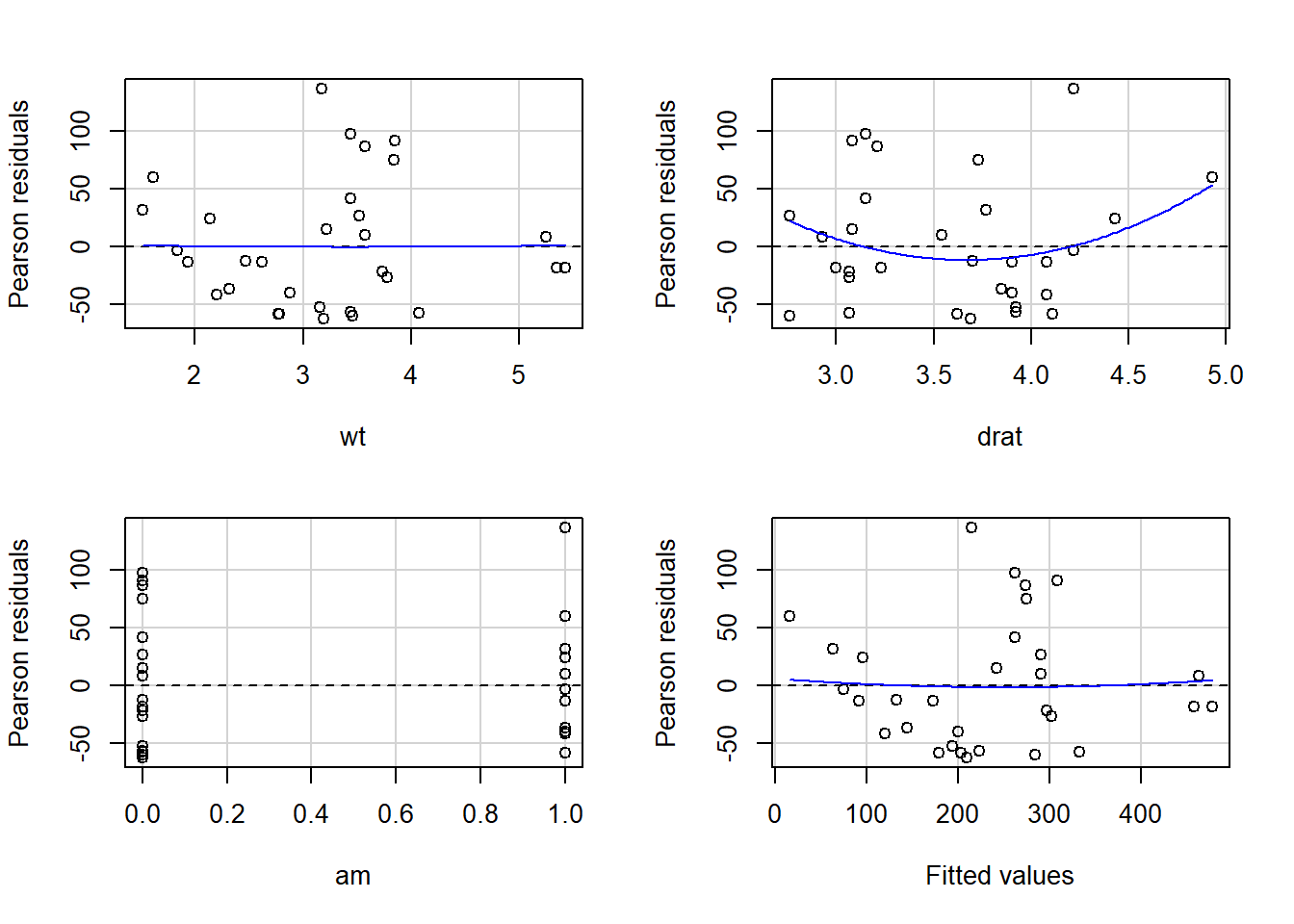

##            Test stat Pr(>|Test stat|)
## wt            0.0467           0.9631
## drat          1.3333           0.1936
## am           -0.1685           0.8675
## Tukey test    0.2071           0.8359

We see above that we received both some scatterplots as well as a table as output. Let’s start with an interpretation of the scatterplots. In the first few scatterplots, the regression residuals have been plotted against each independent variable, one at a time. These plots will help us test the assumption that residual errors are uncorrelated with all independent variables. These scatterplots have fit a blue line to the data. The scatterplot of residuals against wt show a flat line, meaning that the residuals are uncorrelated with wt. However, the scatterplot of residuals against drat shows a curved blue line, meaning that the residuals are not uncorrelated with the residuals. This problem—of drat being correlated with the residuals—is one that we would have to fix before we can trust the results. We will learn how to fix this problem in a later chapter in this textbook. Since am is a dummy variable, the computer does not draw a blue line. Based on our visual inspection, there does not appear to be any relationship between the residuals and the dummy variable am. Remember that if any one independent variable fails this diagnostic test, then the entire test fails and we cannot trust our results for inference.

Note that for our purposes, you can treat a Pearson residual as what we have been calling a residual or a residual error.

Based on our interpretation of the scatterplots above, we can start to fill out the diagnostic tests of assumptions checklist that we drafted earlier:

Completed?	Assumption	Result	Notes
	Residual errors have a mean of 0
	Residual errors are normally distributed
yes	Residual errors are uncorrelated with all independent variables	fail	`drat` failed; other independent variables passed
	All residuals are independent of (uncorrelated with) each other
	Homoscedasticity of residual errors
	Observations are independently and identically distributed
	Linearity of data
	No multicollinearity

Now we can turn to the final scatterplot that we received, which plots residuals against the predicted values (also called fitted values) of our dependent variable from the regression model reg1. This helps us test the linearity of data assumption. We again want the blue line to be flat, such that there is no relationship between the residuals and predicted values. In the plot above, we see that the blue line is almost flat but not quite. This is likely acceptable, but we will turn now to the output table that we received above to continue our diagnostic test of the linearity of data assumption.

In the output table that we received, we see a number of reported test statistics and p-values.¹¹⁰ As always, these p-values are the result of hypothesis tests. In this case, this is a “lack-of-fit”¹¹¹ hypothesis test to tell us if each variable is or is not well-fitted in our OLS regression model.

The hypothesis test for each independent variable is as follows:

$H_0$: The independent variable is linearly related to the dependent variable in the regression model.
$H_A$: The independent variable is non-linearly related to the dependent variable in the regression model.

The hypothesis test above has been conducted for us on each independent variable one at a time. Let’s practice interpreting the results. For wt, the p-value is 0.96, which is very high. This means that for wt, we did not find evidence for the alternate hypothesis that disp and wt are non-linearly related. Therefore, wt passes the test because we did not find any evidence to refute the null hypothesis that disp and wt are linearly related. Now we do the same evaluation for drat. The p-value for drat is 0.19, meaning that there is some limited support for the alternate hypothesis that disp and drat are non-linearly related. Given that we also saw a curved blue line in the scatterplot for drat, this might warrant further investigation, which you will learn how to do in a later chapter in this textbook. Finally, the test for am is also given but is not particularly meaningful since it is a dummy variable.

The very last row of the output table gives us the result of what is called “Tukey’s test for nonadditivity.”¹¹² In this case, the computer conducted a hypothesis test to determine if an alternate possible regression model (different from the OLS model we created) might be a better fit for the data.

Here is a summary of the hypotheses in Tukey’s test for nonadditivity:

$H_0$: Our regression model reg1 fits the data well (linearly, in this case).
$H_A$: A different regression model fits the data better.

To conduct this test, the computer created a different regression model behind the scenes. It then compared our regression model reg1 to this different behind-the-scenes model. The hypothesis test is to help us determine if a) our model reg1 is likely good enough or if b) the behind-the-scenes model is better in which case we should modify reg1. The p-value we received is 0.84, which is very high. This means that we did not find evidence for the alternate hypothesis. We can continue to cautiously assume the null hypothesis, since we did not find any evidence to the contrary from this test.

We are now ready to add to our checklist:

Completed?	Assumption	Result	Notes
	Residual errors have a mean of 0
	Residual errors are normally distributed
yes	Residual errors are uncorrelated with all independent variables	fail	`drat` failed; other independent variables passed
	All residuals are independent of (uncorrelated with) each other
	Homoscedasticity of residual errors
	Observations are independently and identically distributed
yes	Linearity of data	unclear	`drat` is ambiguous; other independent variables passed
	No multicollinearity

We found limited evidence of non-linearity for the independent variable drat. For all other variables and for the model overall, we did not find any other evidence of non-linearity. For the time being, we will note transparently and responsibly that the fit of the variable drat needs to be investigated further, but we will not conduct that further investigation. You will learn how to conduct this investigation in a future chapter.

5.4.3 Normality of residuals in R

The next set of diagnostic tests that we will do will test to see if our regression residuals are normally distributed. This tests the residual errors are normally distributed OLS assumption. We already learned how to test a distribution of data for normality when we tested our t-test samples for normality in a previous chapter. We will use the very same procedure to test our residuals for normality. Below, this entire process is demonstrated but with abbreviated commentary (because the detailed commentary would be exactly the same as the commentary you have already read in the t-test chapter).

Let’s begin by calculating the residuals of our regression model reg1. We already did this earlier in the chapter but will do it again here as well.

This code will calculate the reg1 residuals and add them to our dataset d:

d$resid <- resid(reg1)

We will start by making a histogram of the residuals:

hist(d$resid)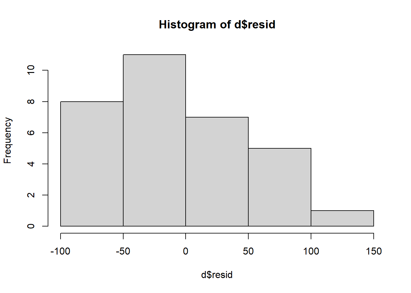

The histogram above follows a normally distributed pattern, but it is cut off on the left side. Preliminarily, this suggests that our residuals are not normally distributed.

Next, let’s make a QQ plot of our residuals:

if (!require(car)) install.packages('car')
library(car)

qqPlot(d$resid)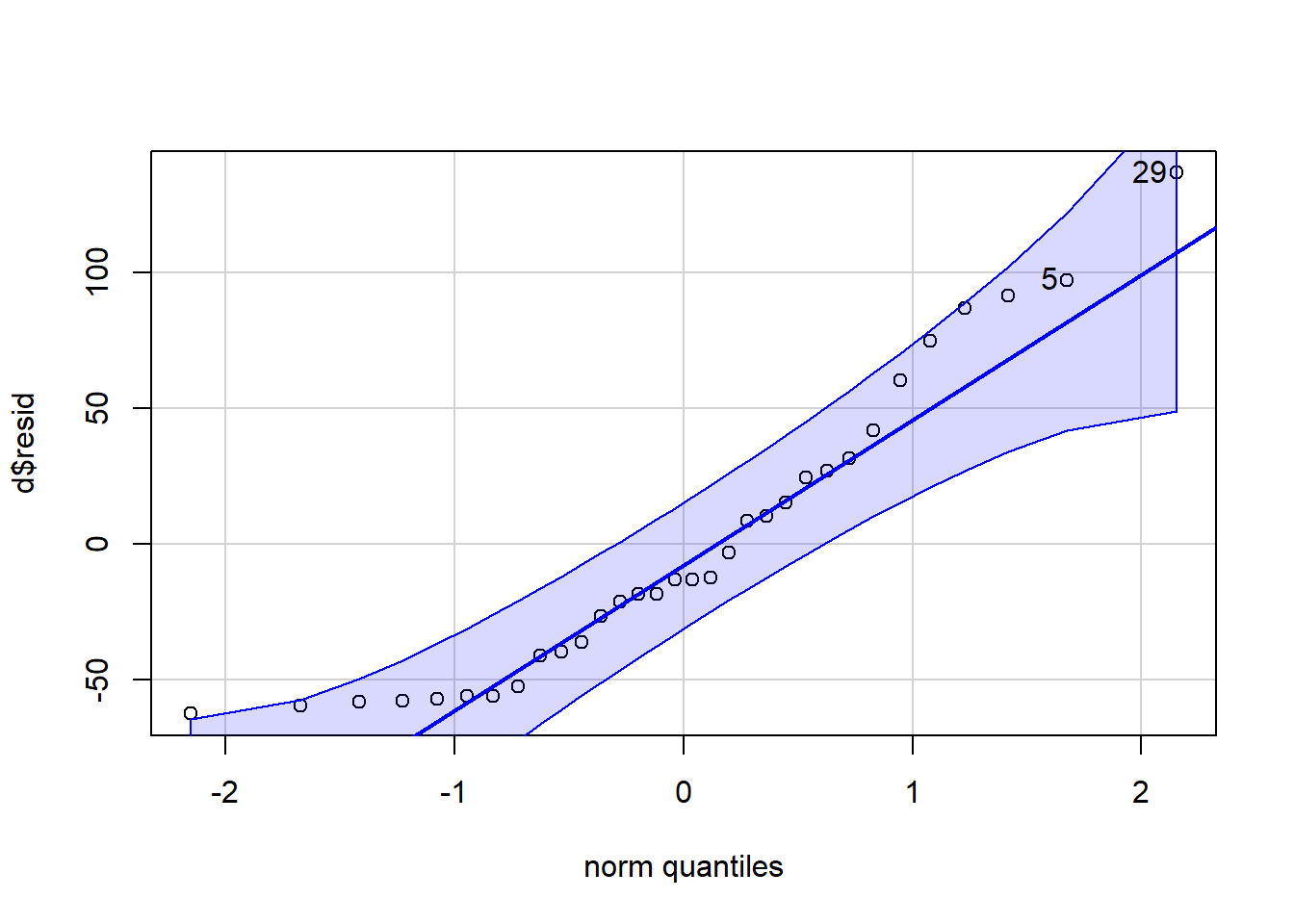

## [1] 29  5

Above, most of the points fall close to the blue line, indicating that they come from a normal distribution. But towards the extreme ends, some of the points start to deviate, with some even falling close to or going over the dotted confidence bands. Overall, this suggests that our data is likely normally distributed. However, we still might want to run our regression a second time after removing some of the observations that fall on the extreme ends of this distribution. Then we could compare the results of reg1 to those of our second regression and see if there are any differences.

Finally, we will conduct a Shapiro-Wilk test on our residuals using the code below:

shapiro.test(d$resid)

## 
##  Shapiro-Wilk normality test
## 
## data:  d$resid
## W = 0.90898, p-value = 0.01057

The extremely low p-value above tell us that our residuals are very likely not normally distributed. Therefore, we cannot trust the results of our OLS model for the purposes of inference.

Let’s continue to fill out our checklist now that we have tested the residuals of reg1 for normality:

Completed?	Assumption	Result	Notes
	Residual errors have a mean of 0
yes	Residual errors are normally distributed	fail
yes	Residual errors are uncorrelated with all independent variables	fail	`drat` failed; other independent variables passed
	All residuals are independent of (uncorrelated with) each other
	Homoscedasticity of residual errors
	Observations are independently and identically distributed
yes	Linearity of data	unclear	`drat` is ambiguous; other independent variables passed
	No multicollinearity

Our checklist is starting to fill out. Let’s keep going, below!

5.4.4 Autocorrelation of residuals in R

We will now test the OLS assumption that all residuals are independent of (uncorrelated with) each other. When we conduct this diagnostic test, we will be testing for what is called autocorrelation. To do this, we will do one visual test and one hypothesis test.

To conduct the visual test, we will look at a scatterplot of the residuals plotted against the row number of each observation, which can be generated using the code below:

plot(seq(1:nrow(d)),d$resid, )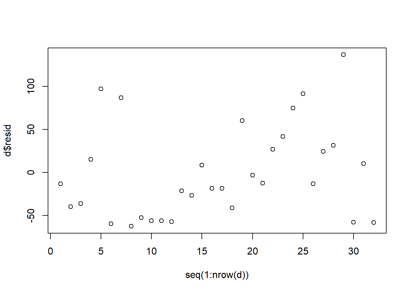

Before we interpret the code above, let’s review what the code we used did:

plot(...) – We want to make a scatterplot.
seq(1:nrow(d)) – This is the first argument we gave to the plot(...) function. This is what will be plotted on the horizontal axis of the scatterplot. What we wanted on the horizontal axis of the scatterplot is simply the row number of each observation. To generate the row numbers as a variable to give to the plot(...) function, we used the seq(...) function. The seq(...) function creates a variable that is a sequence. In this case, we asked it to create a sequence for us from 1 up to the number of rows in the dataset d, which we calculated with the nrow(...) function. We put the nrow(...) function within the seq(...) function within the plot(...) function. To use this code on your own, you can replace d with the name of your own dataset.
d$resid – This is the second argument that we gave to the plot(...) function. This means that we want the variable resid that is within the dataset d to be plotted on the vertical axis of the scatterplot.

In the scatterplot that we received, we are looking for any noticeable pattern in the residuals. Ideally, we would just see complete randomness, with no relationship between residuals that are adjacent to each other. For the most part, we do see fairly random residuals, especially on the right half of the plot (observation 13 and above). However, if we look closely, we also see that observations 8–12 all appear to have almost the same residual. You can find these by looking in the scatterplot where there is a row of points that all have a residual of approximately -50 (on the vertical axis) and row numbers (on the horizontal axis) between 8 and 12. This is evidence of autocorrelation and might be a problem. Let’s dig deeper, below.

Here is a table with our dataset d and all of the variables that are involved in our analysis:

d[c("disp","wt","drat","am","resid")]

##                      disp    wt drat am      resid
## Mazda RX4           160.0 2.620 3.90  1 -13.047902
## Mazda RX4 Wag       160.0 2.875 3.90  1 -39.774061
## Datsun 710          108.0 2.320 3.85  1 -36.142749
## Hornet 4 Drive      258.0 3.215 3.08  0  15.203849
## Hornet Sportabout   360.0 3.440 3.15  0  97.174286
## Valiant             225.0 3.460 2.76  0 -59.713506
## Duster 360          360.0 3.570 3.21  0  86.594051
## Merc 240D           146.7 3.190 3.69  0 -62.519811
## Merc 230            140.8 3.150 3.92  0 -52.555489
## Merc 280            167.6 3.440 3.92  0 -56.149945
## Merc 280C           167.6 3.440 3.92  0 -56.149945
## Merc 450SE          275.8 4.070 3.07  0 -57.114869
## Merc 450SL          275.8 3.730 3.07  0 -21.479990
## Merc 450SLC         275.8 3.780 3.07  0 -26.720413
## Cadillac Fleetwood  472.0 5.250 2.93  0   8.306454
## Lincoln Continental 460.0 5.424 3.00  0 -18.377877
## Chrysler Imperial   440.0 5.345 3.23  0 -18.426025
## Fiat 128             78.7 2.200 4.08  1 -41.193750
## Honda Civic          75.7 1.615 4.93  1  60.254793
## Toyota Corolla       71.1 1.835 4.22  1  -3.433974
## Toyota Corona       120.1 2.465 3.70  0 -12.626194
## Dodge Challenger    318.0 3.520 2.76  0  26.997986
## AMC Javelin         304.0 3.435 3.15  0  41.698329
## Camaro Z28          350.0 3.840 3.73  0  74.684595
## Pontiac Firebird    400.0 3.845 3.08  0  91.174514
## Fiat X1-9            79.0 1.935 4.08  1 -13.119506
## Porsche 914-2       120.3 2.140 4.43  1  24.456471
## Lotus Europa         95.1 1.513 3.77  1  31.477865
## Ford Pantera L      351.0 3.170 4.22  1 136.546721
## Ferrari Dino        145.0 2.770 3.62  1 -57.978543
## Maserati Bora       301.0 3.570 3.54  1  10.114863
## Volvo 142E          121.0 2.780 4.11  1 -58.160229

Above, if we count down to the 8th, 9th, 10th, 11th, and 12th rows, we see that all of those cars are Merc cars. And all of them have a residual of approximately -50. This is unacceptable. This means that there is non-randomness in our residuals. This means that we should not necessarily trust our OLS results for the purposes of inference. This also uncovers a potential problem with our research design. What population does this sample represent? Can we reasonably say that this sample represents all cars? Probably not. When we do inference, we have to be mindful not only of the diagnostic tests that we do in R but also of how our research design and sampling strategy might influence our results.

Anyway, with some possible visual evidence of autocorrelation in mind, let’s turn to a hypothesis test that can help us further investigate. We will run the Durbin-Watson test for autocorrelation.

Here are the hypotheses for the Durbin-Watson test:

$H_0$: Residuals are not autocorrelated.
$H_A$: Residuals are autocorrelated.

And here is how we run the Durbin-Watson test in R:

if (!require(lmtest)) install.packages('lmtest')
library(lmtest)

dwtest(reg1)

## 
##  Durbin-Watson test
## 
## data:  reg1
## DW = 1.8701, p-value = 0.2462
## alternative hypothesis: true autocorrelation is greater than 0

In the code we ran above, we first installed the lmtest package if necessary, loaded the lmtest package, and then ran the dwtest(...) function with our regression model reg1 as an argument in that function. This ran the hypothesis test for us.

The resulting p-value of 0.25. Is not strong enough to worry us about autocorrelation as a result of the Durbin-Watson test in and of itself. Of course, since we found visual and theoretical evidence of possible autocorrelation due to the Merc observations, we will still consider our OLS model reg1 to have failed the autocorrelation diagnostic test.

Let’s add to our OLS diagnostics checklist:

Completed?	Assumption	Result	Notes
	Residual errors have a mean of 0
yes	Residual errors are normally distributed	fail
yes	Residual errors are uncorrelated with all independent variables	fail	`drat` failed; other independent variables passed
yes	All residuals are independent of (uncorrelated with) each other	fail
	Homoscedasticity of residual errors
	Observations are independently and identically distributed
yes	Linearity of data	unclear	`drat` is ambiguous; other independent variables passed
	No multicollinearity

Before we conclude our study of autocorrelated residuals, let’s see an extreme example of what problematic autocorrelation would look like. Have a look at the scatterplot below of hypothetical residuals plotted against hypothetical observations, from another hypothetical regression.

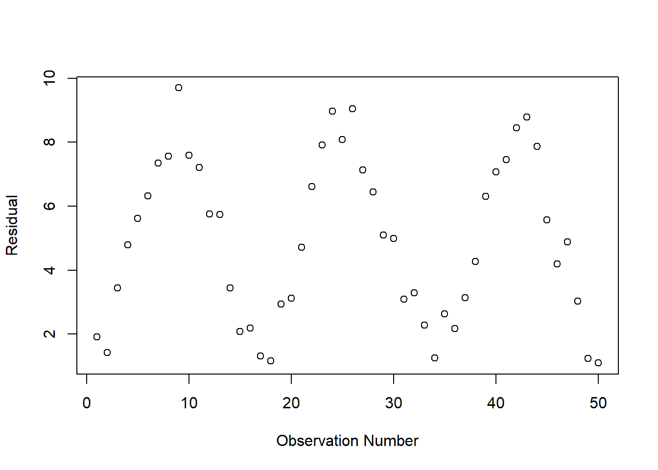
Above is an example of extreme autocorrelation. Each observation’s residual is very close to the residual of the previous observation. The residuals are not random at all. Each residual is likely related to the residual before and after it. Residuals that appear like this indicate a potential problem that require further investigation.

5.4.5 Homoscedasticity of residuals in R

Another OLS assumption is homoscedasticity of residual errors. The diagnostic tests for this assumption are also conducted both as a visual examination and a hypothesis test. We will begin with a visual test. We will conduct this visual test by looking at a scatterplot that we have already seen once before: the plot of the residuals plotted against the predicted values. This was part of the output that we received when we ran the residualPlots(...) command earlier in the chapter.

Remember:

Homoscedasticity of the residuals is good and what we ideally want to find.
Heteroskedasticity is bad, what we ideally don’t want to find.

Here is a copy of the residuals plotted against predicted values, so that you don’t have to go up to look at it again:

if (!require(car)) install.packages('car')
library(car)

residualPlots(reg1, ~1, fitted=TRUE)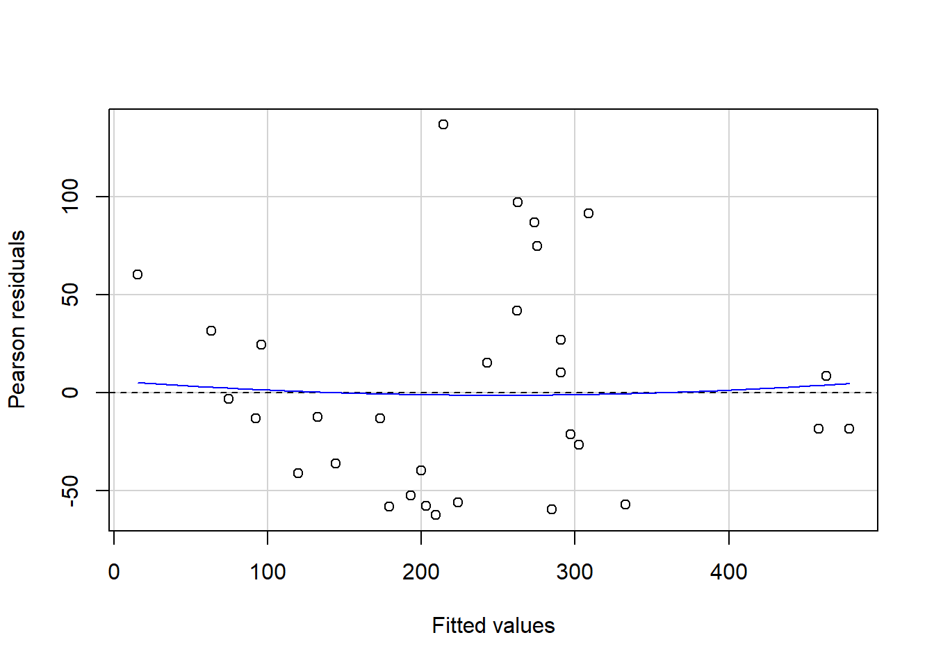

##            Test stat Pr(>|Test stat|)
## Tukey test    0.2071           0.8359

This time, we are looking in the scatterplot above to see if there is any noticeable pattern in the variance—or spread—of the residuals. Ideally, we would see complete randomness, with the residuals spread out fairly evenly around the horizontal black dotted line as we look across the scatterplot horizontally. This would indicate that the residuals are evenly distributed. If we instead see a noticeable pattern in the residuals across the predicted values, that would indicate a problem. In this case there does not appear to be any kind of pattern. So far, we can probably safely assume that our residuals are homoscedastic, meaning that they have constant variance. If we had noticed a pattern, then we would instead refer to our residuals as heteroscedastic, which would be a violation of the OLS assumptions.

Let’s turn to the hypothesis test of homoscedasticity. This is called the Breusch-Pagan test. For the Breusch-Pagan test, we have the following hypotheses:

$H_0$: The variance of the residuals is constant. The residuals are homoscedastic.
$H_A$: The variance of the residuals is not constant. The residuals are heteroscedastic.

if (!require(car)) install.packages('car')
library(car)

ncvTest(reg1)

## Non-constant Variance Score Test 
## Variance formula: ~ fitted.values 
## Chisquare = 0.005343423, Df = 1, p = 0.94173

Above, we yet again loaded the car package first. We then ran the ncvTest(...) function with our regression model reg1 as the argument within that function. This code conducted a Breusch-Pagan test.

The p-value of 0.94 shows that there is no evidence of heteroscedasticity in our regression model reg1. Since both visual inspection and the Breusch-Pagan test did not show any evidence of heteroscedasticity, we can conclude that our model reg1 passes this diagnostic test and does not violate the OLS assumption of homoscedasticity of residual errors.

Let’s add this diagnostic test result to our checklist:

Completed?	Assumption	Result	Notes
	Residual errors have a mean of 0
yes	Residual errors are normally distributed	fail
yes	Residual errors are uncorrelated with all independent variables	fail	`drat` failed; other independent variables passed
yes	All residuals are independent of (uncorrelated with) each other	fail
yes	Homoscedasticity of residual errors	pass
	Observations are independently and identically distributed
yes	Linearity of data	unclear	`drat` is ambiguous; other independent variables passed
	No multicollinearity

Before we conclude our examination of homoscedasticity, let’s look at an example of what clear heteroscedasticity would look like. Have a look at the example scatterplot below of hypothetical residuals plotted against hypothetical predicted values from a hypothetical regression model.

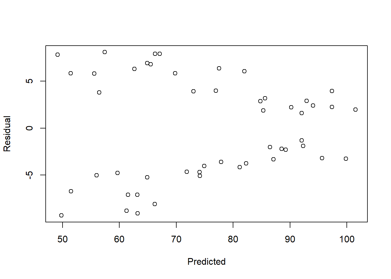
Above, we see that the residuals fall into what we could call a cone shape. The wide base of the cone is on the left and the narrow top of the cone is on the right. The variance—or spread—of the residuals is large at low predicted values (on the left side of the plot) and small at higher predicted values (on the right side of the plot). If we had found residuals like we see in the plot above, we would conclude that our residuals are heteroscedastic. A regression model with heteroscedastic residuals violates the homoscedasticity OLS assumption and cannot be trusted for inference.

5.4.6 Multicollinearity detection in R

Now it is time to discuss an OLS assumption that does not relate to the residuals: no multicollinearity. Multicollinearity is a diagnostic test that relates only to the independent variables in a regression model. Multicollinearity is a problem that occurs in an OLS model when the independent variables are too highly correlated with each other. Testing for multicollinearity has nothing to do with the dependent variable or the residuals of a regression model.

The first step is to simply look at the correlation of the independent variables in our regression models. One way to do this is to make a copy of our dataset d called d.partial that only contains our three independent variables.

Below, we create d.partial with only our three independent variables wt, drat, and am:

d.partial <- d[c("wt","drat", "am")]

Next, we can run the same cor(...) function that we have used before, but this time with our dataset d.partial as the function’s only argument:

cor(d.partial)

##              wt       drat         am
## wt    1.0000000 -0.7124406 -0.6924953
## drat -0.7124406  1.0000000  0.7127111
## am   -0.6924953  0.7127111  1.0000000

Above, the computer created a correlation matrix for us. It calculated the correlation of each variable in the dataset d.partial with every other variable in the dataset. For example, we see that wt and drat are correlated with each other at -0.71.

We can also once again create a fancier version of this correlation matrix with the following code which you learned about earlier in this chapter:

if (!require(PerformanceAnalytics)) install.packages('PerformanceAnalytics')
library(PerformanceAnalytics)

chart.Correlation(d.partial, histogram = TRUE)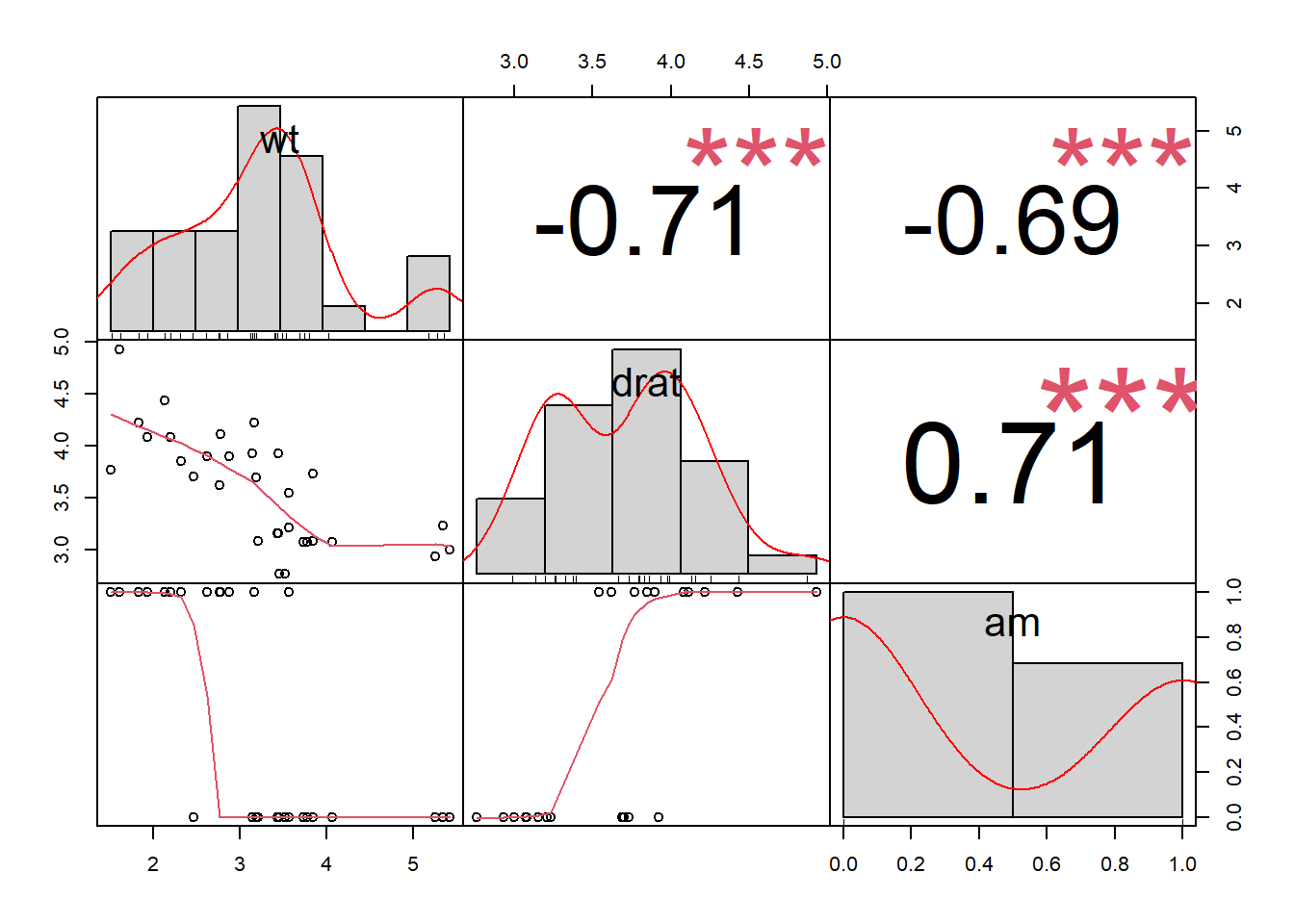

Now that we have generated both plain and fancy versions of our correlation matrix, let’s get down to analyzing this output to check for multicollinearity. When the problem of multicollinearity is present, that means that the independent variables are too highly correlated with each other. The problem of multicollinearity can cause the hypothesis test for each slope calculation in the OLS regression to be conducted incorrectly. When multicollinearity is a present, the p-value and confidence interval for each slope estimate may not be trustworthy. In the correlation matrix above, all of the variables are highly correlated with each other. Remember: the maximum amount of correlation possible is either -1 or +1. -1 is a very high negative correlation and +1 is a very high positive correlation. The correlations we see above are all very close to either -1 or +1, meaning that multicollinearity may be a problem in our regression model reg1.

In the example above, all of the independent variables are highly correlated with each other. However, note that even if any two independent variables are highly correlated with each other, that is cause for concern and you should consider removing one of those independent variables from the regression model, if possible.

The next way to test for multicollinearity is by looking at the VIF—variance inflation factor—of each independent variable in our OLS regression model.

Here is the code we use to do the VIF test:

if (!require(car)) install.packages('car')
library(car)

vif(reg1)

##       wt     drat       am 
## 2.363655 2.500118 2.365507

In the code above, we loaded the car package and then ran the vif(...) function with reg1 as the function’s argument. The computer then gave us VIF values for each independent variable. Note that these are not p-values or confidence intervals. These are something different. They are VIF values.

When a variable has a VIF value of 4 or more, that indicates that multicollinearity might be a problem in our regression model. All of these VIF values are under 4, so we can say that our OLS model reg1 passes the VIF test. However, we cannot ignore the very high correlation of the independent variables that we saw earlier. Typically, such high correlations would be too high and we would adjust our regression model by removing one or more independent variables and running it again. There are also more complicated methods that can be used to resolve multicollinearity, but these are beyond the scope of this textbook.

Any time you find high correlations among any two or more independent variables or high VIF values, you should first try removing an independent variable from your regression model and running the regression again. There are also other, more advanced ways to fix multicollinearity which do not involve removing one or more variables from your regression model.¹¹³ Often, these more advanced approaches are not necessary. These approaches are beyond the scope of this textbook.

We are now ready to add our result of the no multicollinearity OLS diagnostic test to our checklist:

Completed?	Assumption	Result	Notes
	Residual errors have a mean of 0
yes	Residual errors are normally distributed	fail
yes	Residual errors are uncorrelated with all independent variables	fail	`drat` failed; other independent variables passed
yes	All residuals are independent of (uncorrelated with) each other	fail
yes	Homoscedasticity of residual errors	pass
	Observations are independently and identically distributed
yes	Linearity of data	unclear	`drat` is ambiguous; other independent variables passed
yes	No multicollinearity	unclear	VIF passed but correlations are very high

5.4.7 Mean of residuals

Another OLS assumption is that the residual errors have a mean of 0. We already calculated the residuals of our regression model reg1 and added them to our dataset d as the variable resid. So, let’s just go ahead and see what the mean of these residuals is.

This code calculates the mean of the reg1 residuals:

mean(d$resid)

## [1] -1.554312e-15

Above, we see that the mean of the residuals is an extremely small number. This is basically 0. In fact, in OLS, the mean of the residuals of our regression model is always 0. That is how OLS linear regression is programmed. The math used to calculate OLS linear regression results require that the mean of the residuals is 0. Therefore, this is not an assumption that we can test. As you read earlier, the residual errors should have a population mean of 0.¹¹⁴ This means that our test of this assumption is more theoretical than anything else. We have to ask ourselves: is there anything about our sampling method, the population from which we are sampling, our research design as a whole, or any other factor that might cause our regression residuals to be non-random? If the regression residuals are random, their population mean will be 0. If something is causing the residuals to be non-random, then the population mean of the residuals may not be random and the OLS assumption that the residual errors have a mean of 0 would be violated and we could not trust our regression results to conduct inference.

For now, since we do not know much about how the cars in our dataset were sampled, let’s conclude that we don’t know for sure if the population mean of our residuals is 0 or not. That is what we will write into our checklist.

Here is an updated copy of our checklist:

Completed?	Assumption	Result	Notes
yes	Residual errors have a mean of 0	unclear	Inadequate information about research design
yes	Residual errors are normally distributed	fail
yes	Residual errors are uncorrelated with all independent variables	fail	`drat` failed; other independent variables passed
yes	All residuals are independent of (uncorrelated with) each other	fail
yes	Homoscedasticity of residual errors	pass
	Observations are independently and identically distributed
yes	Linearity of data	unclear	`drat` is ambiguous; other independent variables passed
yes	No multicollinearity	unclear	VIF passed but correlations are very high

5.4.8 Independence of observations

Only one diagnostic test remains, the test of the OLS assumption that observations are independently and identically distributed (this is often called the “IID” assumption). We will use our knowledge of theory and research design to test this assumption. To satisfy this assumption and pass this diagnostic test, observations in our data should not influence each other in any way or have measurable characteristics that are related to each other in any way. For example, if we are sampling 100 people to test how well they do on a test, if some students work together in groups instead of working alone to answer the test questions, their results are not independent of each other. Students who worked in groups together influenced each other’s results.

In our example analysis for which we created the OLS regression model reg1, we do not have sufficient knowledge about how the observations in our dataset d were selected. If they were selected non-randomly, then we likely violate the IID assumption. Typically, if we have a reliable sampling strategy that randomly samples observations into a dataset from the population of interest, we will satisfy the IID assumption of OLS.

For now, we will complete our checklist in a way that reflects our uncertainty about the IID assumption for reg1:

Completed?	Assumption	Result	Notes
yes	Residual errors have a mean of 0	unclear	Inadequate information about research design
yes	Residual errors are normally distributed	fail
yes	Residual errors are uncorrelated with all independent variables	fail	`drat` failed; other independent variables passed
yes	All residuals are independent of (uncorrelated with) each other	fail
yes	Homoscedasticity of residual errors	pass
yes	Observations are independently and identically distributed	unclear	Inadequate information about research design
yes	Linearity of data	unclear	`drat` is ambiguous; other independent variables passed
yes	No multicollinearity	unclear	VIF passed but correlations are very high

It is important to make sure that your research design is appropriate for the question you are trying to answer. If the question you are trying to answer will be answered using an OLS regression model that analyzes a sample to make an inference about a population, your research/project design should be such that the IID assumption of OLS is definitely satisfied. You should also try to maximize the chances that most other OLS assumptions will also be satisfied. Of course, this might not always be possible. A large portion of the remainder of this textbook is devoted to creating regression models that are more appropriate than OLS linear regression for situations in which our research design and/or data violate the OLS assumptions and fail to pass the diagnostic tests that we have just reviewed.

5.4.9 Conclusion of diagnostic testing

We have now completed all of the diagnostic tests of OLS assumptions that must be conducted before an OLS regression result can be trusted for the purposes of inference. As you practice, you will become more and more used to conducting these tests after every regression model you run. It may seem like a lot of tests now, but if you repeat these tests on many different datasets and regression models, you will develop speed and comfort. You will also develop your own library of R commands that you save within your own RMarkdown files that you can quickly find and modify each time you work on a new project. This is why it is important for all of your quantitative analysis work to be saved carefully and coded in a reproducible way.

In the example presented in this chapter, our regression model reg1 failed most of the diagnostic tests. Therefore, it would be irresponsible for us to make claims about an entire population of automobiles based on this sample of 32 automobiles. Our regression results do tell us on average what is happening within our sample alone, but they do not tell us anything trustworthy about a population.

Finally, one topic that is not discussed in this chapter is analysis of outliers. The presence of outliers in our data may sometimes cause our regression model to violate some of the OLS regression assumptions. Sometimes, only if it is reasonable to do so, we can remove one or more outliers from our data before running a regression. The most responsible thing to do is to run our regression with and without any outliers and see if we get the same results both times. If we do get similar results each time, we can be more confident about our results. If we do not get similar results each time, we should hesitate to make a definitive conclusion and instead report exactly what happened (that we got conflicting or inconclusive results). Alternatively, if we do not get similar results each time, we should have a strong justification for choosing one regression result over another.

There are many techniques can be used to identify outliers. However, outlier identification is beyond the scope of this chapter.

5.4.10 What to do when diagnostic tests fail

We know from the content earlier in the chapter that when our regression results fail one or more diagnostic tests, we cannot trust our results. So what do we do next to answer our research question? Many of the analytic techniques covered later in this book help us answer this question. Solutions include squaring one or more independent variables, matching to reduce model dependence, and multilevel modeling using fixed or random effects. Another option that we have already briefly discussed is to transform.

However, there are a few classic fixes that you can also attempt right away:

Log-transform the dependent variable and/or one or more independent variables. To do this, remove the variable that is potentially causing problems and replace it with a log-transformed version of itself in the regression model.
Square root transform the dependent variable and/or one or more independent variables. Again, to do this, remove the variable that is potentially causing problems and replace it with a transformed version of itself in the regression model.
Transform a continuous numeric variable into dummy variables, based on selected intervals of the numeric variable. For example, if you have an age variable which records how old each observation (person) is, you can convert this into separate dummy variables to indicate five or ten-year age groups. If you have people in your sample with ages 21–50 years, you could create three dummy variables, one for people ages 21–30 years, another for 31–40 years, and another for 41–50 years. You would then exclude the continuous numeric age variable from your regression model and include two of the three new dummy variables.

After making one or more of the changes above to your regression model and variables, you would again run all diagnostic tests on the new regression model to see if it passes the tests. If it does pass the test and if your regression model is still reasonably analyzing your data, you can then trust the results.

Note that the strategies above are not only applicable to OLS regression. These techniques to modify regressions can also be used in most of the other types of regression models that we will study together.

5.5 Summary of regression research process

In general, the overall process we should follow when using OLS and other regression methods to do research or a project is:

Ask a question that we want to answer using numbers.
Gather and/or prepare the appropriate data to answer the question.
Run the appropriate regression model.
Examine goodness-of-fit.
Run diagnostic tests of regression model assumptions to determine if we can or cannot trust our regression results.
Make any necessary modifications to data and/or regression model specification and then repeat steps above as many times as necessary.
If goodness-of-fit and diagnostic tests results are satisfactory, carefully interpret regression results and cautiously make conclusions.
Transparently report the entire process and results.

5.6 Dummy variables again

In this section, we revisit the concept of a dummy variable. The video below demonstrates how dummy variables are created and then used in a regression analysis. You are not required to watch the entire video, but I recommend that you at least skim it to see if it would be useful to you to watch it all. It demonstrates the entire process of running a regression analysis, with a heavy focus on the use of dummy variables to include qualitative data in quantitative analysis (which is the entire purpose of dummy variables in our study of statistics).

The video above can also be viewed externally at https://youtu.be/cYMNEznBDCg.

As you now know, “dummy” variables are variables that just have two values. Here are some examples:

Variable	Levels
gender	female, male
experimental group	treatment, control
completed training	did complete training, did not complete training
citizenship	native, foreign
test result	pass, fail
transmission type	automatic, manual

How does this look within a dataset? Maybe you would have a variable in your dataset called gender and it would be coded as 1 for females and 0 for males. Note that constructs like gender are qualitative. Male and female are not numeric concepts. By converting them into 1 and 0, we made them numeric. This is analogous to how we incorporated and interpreted the am variable in our reg1 example earlier in this chapter.

A dummy variable can also be called a binary variable, dichotomous variable, yes/no variable, two-level categorical variable, or anything similar. All of these terms mean the same thing. For our purposes, it is simply a variable that can have a value of 0 or 1, and nothing else.

But what about when you have three or more qualitative (non-numeric) categories that you want to include in your regression as a single variable?

Here are some examples:

Variable	Levels
Race	black, white, other
Favorite ice cream flavor	chocolate, vanilla, strawberry, other
Type of car owned	Gas, electric, hybrid, do not have a car

Let’s add a qualitative variable with three or more categories to the dataset d—which is a copy of mtcars—that we were using earlier. We will call this new variable region, to indicate what part of the world a car was made in.

Here, we add the region variable to d:

d$region <- c("asia","asia","asia","northamerica","northamerica","northamerica","northamerica","europe","europe","europe","europe","europe","europe","europe","northamerica","northamerica","northamerica","europe","asia","asia","asia","northamerica","northamerica","northamerica","northamerica","europe","europe","europe","northamerica","europe","europe","europe")

Now the dataset d has a new variable called region. The variable region has three levels: asia, northamerica, and europe. region is a categorical variable. How can we possibly analyze it quantitatively?

Well, one option is to make a boxplot:

boxplot(disp ~ region, data = d)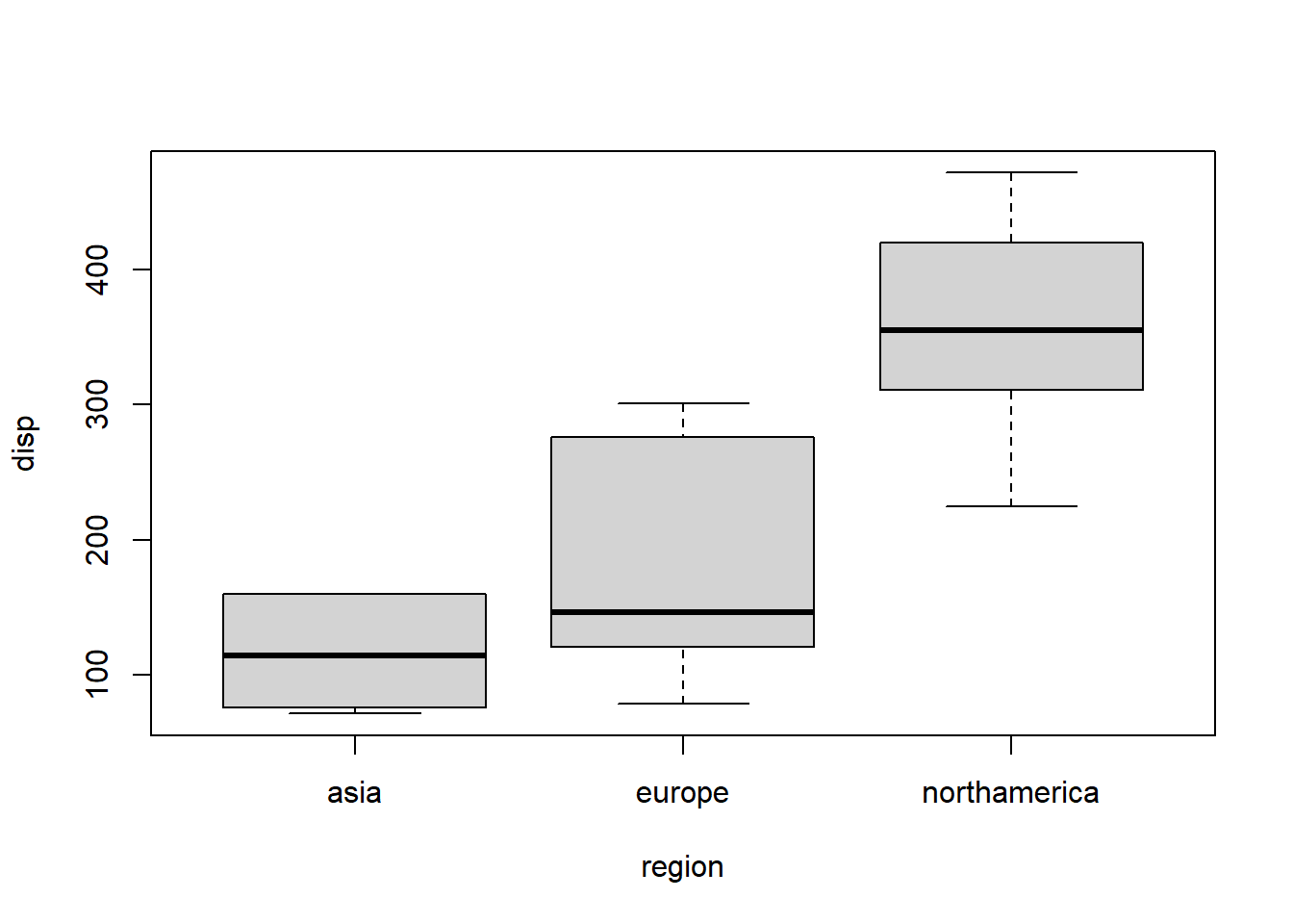

Above, we see that disp, our dependent variable of interest, seems to be quite different across cars from the three different regions. Now we want to examine this relationship in a regression analysis where we can control for other variables. Let’s set up our research design.

Research design:

Question of interest: Does displacement differ in cars from different regions?
Data: copy of mtcars data called d
Analytic method: OLS
Dependent variable: disp
Independent variables: wt, drat, am, region

We are almost ready to run a regression. We know what question we want to answer, we have our data and variables. But one variable—region—is not numeric. How can we make it numeric so that we can put it into our OLS regression? We will have to create multiple dummy variables to help identify each observation.

The code below creates dummy variables for us for the variable d$region:

if (!require(fastDummies)) install.packages('fastDummies')
library(fastDummies)

d <- dummy_cols(d,select_columns = c("region"))

Here’s what the code above did:

Load fastDummies package. This is a package that is specifically designed to help us quickly turn a qualitative categorical variable like region into dummy variables.
d <- – Replace the dataset d with a new version of d that is created by the dummy_cols(...) function.
dummy_cols(d,select_columns = c("region")) - Run the dummy_cols(...) function which will turn a categorical variable into multiple dummy variables. This function has two arguments:
- d – This is the dataset that is being used.
- select_columns = c("region") – This tells the computer which variables in the original dataset d we want to turn into dummy variables. In this case, region is the only one we have specified, but we could add others too if we wanted.

Let’s inspect the new version of d. You can do this by running View(d) on your computer. Three new dummy variables were generated, called region_europe, region_asia, and region_northamerica.

Below is an example of three observations (cars) selected from the data, one from each region:

region	region_europe	region_asia	region_northamerica
northamerica	0	0	1
europe	1	0	0
asia	0	1	0

Let’s go through an example: The first car is from North America. Its region, the qualitative variable, was coded as northamerica. In our three dummy variables, it is coded as 0 for region_europe and region_asia. It is coded as 1 for region_northamerica.

Now let’s remove the first column from the table:

region_europe	region_asia	region_northamerica
0	0	1
1	0	0
0	1	0

Using just the dummy variables in the table above, we can tell that the first car is from North America, the second car is from Europe, and the third car is from Asia. And now we are doing it all using numbers and all using variables that are coded as either 0 or 1! We turned the qualitative categorical variable region, which had three levels, into three dummy variables which each have two levels (0 and 1).

Now we can make a regression model to answer our question:¹¹⁵

reg2 <-  lm(disp~wt+drat+am+region_europe+region_asia, data = d)

Above, we made a regression model that we saved as reg2. The dependent variable is disp. The independent variables are wt, drat, am, region_europe, and region_asia. Note that we left out region_northamerica from the list of independent variables. You always have to leave out one dummy variable from the regression for any particular qualitative categorical variable. In this case, the qualitative categorical variable region led to the creation of three dummy variables; one of those dummy variables must be left out of the regression. The category that is left out of the regression is called the reference category. Above, North American cars are the reference category. Let’s have a look at our regression results:

if (!require(jtools)) install.packages('jtools')
library(jtools)

summ(reg2, confint = TRUE)

Observations	32
Dependent variable	disp
Type	OLS linear regression

F(5,26)	59.98
R²	0.92
Adj. R²	0.90

	Est.	2.5%	97.5%	t val.	p
(Intercept)	69.47	-120.37	259.31	0.75	0.46
wt	86.18	62.83	109.53	7.59	0.00
drat	-17.49	-60.96	25.99	-0.83	0.42
am	39.53	-4.14	83.19	1.86	0.07
region_europe	-109.92	-147.60	-72.24	-6.00	0.00
region_asia	-112.38	-165.86	-58.91	-4.32	0.00
Standard errors: OLS

The equation for this regression model is:

\[\hat{y} = 86.18wt - 17.49drat + 39.53am -109.92region\text{_}europe -112.38region\text{_}asia + 69.47\]

The predicted value of disp for a car that weighs 1.5 tons, has a rear axle ratio of 2 units, has an automatic transmission, and was made in Asia would be calculated like this:

$\hat{y} = (86.18*1.5) - (17.49*2) + (39.53*0) - (109.92*0) -(112.38*1) + 69.47 = 51.38 \text{ cubic inches}$

If this same car was instead made in North America, we would calculate its predicted disp like this:

$\hat{y} = (86.18*1.5) - (17.49*2) + (39.53*0) - (109.92*0) -(112.38*0) + 69.47 = 163.76 \text{ cubic inches}$

In this regression model, we would interpret wt, drat, and am the same way we did earlier in the chapter. Let’s focus just on our two new dummy variables, region_europe and region_asia.

Interpretation of region dummy variables, in our sample:

Cars that are made in Europe are predicted on average to have displacement that is 109.92 cubic inches lower than displacement of cars made in North America, controlling for all other independent variables.
Cars that are made in Asia are predicted on average to have displacement that is 112.38 cubic inches lower than displacement of cars made in North America, controlling for all other independent variables.

Interpretation of region dummy variables, in the population from which our sample was drawn:

We are 95% confident that cars that are made in Europe have on average a displacement that is between 147.60 and 72.24 cubic inches lower than displacement of cars made in North America, controlling for all other independent variables.
We are 95% confident that cars that are made in Asia have on average a displacement that is between 165.86 and 58.91 cubic inches lower than displacement of cars made in North America, controlling for all other independent variables.
These results are of course only trustworthy if our model and data pass all diagnostic tests and satisfy all OLS assumptions.

Importantly, notice that the regression results for these region dummy variables can only tell us how European and Asian cars compare to North American cars. They can NOT tell us how European and Asian cars compare to each other. This is because we decided to leave out the North American cars dummy variable from the regression and designate it as the reference category. If we had wanted, we could have left out one of the other regions as the reference category. if we had left Europe out of the regression and we had included Asia and North America, then we would be comparing the displacement of Asian and North American cars to that of European cars.

You might be wondering: Why can’t we just include all three dummy variables in the regression? The reason we cannot do this is because doing so would violate at least one OLS regression assumption. We cannot include variables that are perfect linear combinations of each other. In fact, the computer would not even allow you to do so. It would remove one of the three variables for you from the regression model. One way to think about it is like this: Once the computer knows whether a car is Asian or not and it also knows if that car is European or not, it definitely knows already if that car is North American or not. You don’t need to explicitly tell the computer. Therefore, just two of the dummy variables are enough for the computer to know everything about your data related to the region variable. Adding in the third dummy variable would be redundant, unnecessary information.

In all cases, we include one dummy variable fewer than the number of categories in the qualitative categorical variable that we are trying to analyze:

\[number\; of\; dummy\; variables = number\; of\; categories - 1\]

Also, keep in mind that the computer “thinks” that the variables region_asia and region_europe are continuous numeric variables. It does not know that these variables can only have a value of 0 or 1. The same is the case for the am variable, as we discussed earlier in the chapter.

As you continue to learn more about quantitative analysis, you are likely to run into situations where you need to do quantitative analysis on qualitative data. The strategy of dividing qualitative categorical data into dummy variables can be very handy and it is a good skill to practice. We will be using dummy variables repeatedly in the rest of this textbook for a variety of useful purposes.

5.7 Assignment

In this chapter’s assignment, you will use a single dataset to run a multiple OLS linear regression model. The analysis you conduct should be extremely thorough and go step-by-step through the entire research process as you would do when using OLS to answer a research question. You can definitely use your own data instead of the provided data for this assignment, if you prefer. If you do use your own data, it must contain at least one qualitative categorical variable with three or more possible values/levels.

To get started, first load the hsb2 data using the following code:

if (!require(openintro)) install.packages('openintro')
library(openintro)

data(hsb2)
h <- na.omit(hsb2)

You should also run the command ?hsb2 in the console to read more about the dataset, which is called the High School and Beyond survey.¹¹⁶

You will use h as your dataset for this portion of the assignment, NOT hsb2. h is a copy of the dataset hsb2 in which any missing data was removed using the na.omit(...) function.

You will conduct a quantitative analysis with the following characteristics:

Question: What is the relationship between the outcome science and: gender, ses, prog, write, and socst?
Data: hsb2 (copied as h)
Dependent variable: science
Independent variables: gender, ses, prog, write, and socst
Analysis method: OLS

If you choose to use your own separate data, make sure to include and explain all of the characteristics above as part of the assignment you submit.

5.7.1 Prepare and explore the data

We’ll start with a few tasks to modify the data a little bit so that it is ready for you to analyze. You will also explore the data using techniques you have learned before, before you move on to running a regression model.

Task 1: Run the command summary(h) to start to learn about this dataset.

Task 2: Make a list of the six variables that will be used in this analysis. Note down which ones are continuous numeric, which ones are qualitative categorical, and/or which ones are something else.

Task 3: Convert the ses variable into a new quantitative continuous numeric variable with a different name, according to the table below. Use the new quantitative variable in all analyses, not the original ses variable. Note that this task is NOT asking you to make dummy variables. It is asking you to recode a variable the way you learned earlier in the course. You will make dummy variables later in this assignment, though!

Level of already-existing `ses` variable	Level of new quantitative variable
low	1
middle	2
high	3

ses is no longer a qualitative categorical variable in your analysis.

Task 4: Create a two-way table to show that you created the new version of the ses variable successfully.

Task 5: Make boxplots to show how science varies across the values of all categorical variables of interest. Interpret any trends or noteworthy observations you see. Note that you will make a separate boxplot for each categorical independent variable.

Task 6: Make a correlation matrix with all numeric variables involved in our study. Interpret any trends or noteworthy observations you see.

Task 7: For all categorical variables, use the dummy_cols function in the fastDummies package to create appropriate dummy variables. Note that ses is not a categorical variable anymore since we changed it to a numeric variable above, so do not make dummy variables for SES.

5.7.2 Multiple OLS linear regression

In this section, you will run an OLS regression to answer the question of interest. You will then interpret the results in both the sample and population.

Task 8: Run the appropriate OLS regression model and show the results. Please include in the model: a) any relevant numeric independent variables, b) the correct dummy variables corresponding to any relevant categorical independent variables, which you should have created earlier in the assignment.

Task 9: Write the regression equation.

Task 10: Calculate the predicted value of the dependent variable for somebody with the following characteristics: female, level 2 socioeconomic status, vocational program, 50 standardized writing score, 38 standardized social studies score.

Task 11: Interpret regression results for each independent variable for your sample.

Task 12: Interpret regression results for each independent variable for the population.

Task 13: List two ways that you could calculate $R^2$ for this regression model (but don’t actually calculate them; just say what the two possible approaches are).

Task 14: Pick one of the ways of calculating $R^2$, whichever one you prefer, and show the entire process of calculating it that way.

5.7.3 Diagnostic tests of OLS assumptions

Now you will run and interpret all required diagnostic tests for the OLS regression model that you created earlier in the assignment.

Task 15: Make an empty checklist of the OLS diagnostic tests on a piece of paper, so that you can check off tests as you do them.¹¹⁷ You do not need to submit this checklist.

Task 16: Conduct and show/explain the results of ALL diagnostic tests for multiple OLS. Your answer to this task will likely be quite long and have multiple sections.

Task 17: In 3–5 sentences, write a short conclusion in which you address our question of interest, taking into account all of the evidence you generated.

5.7.4 Additional items

You have now reached the end of this week’s assignment. The tasks below will guide you through submission of the assignment, remind you of any other items you need to complete this week, and allow us to gather questions and/or feedback from you.

Task 18: You are required to complete 15 quiz question flashcards in the Adaptive Learner App by the end of this week.

Task 19: Please write any questions you have for the course instructors (optional).

Task 20: Please write any feedback you have about the instructional materials (optional).

Task 21: If you already know your schedule, please email Anshul and Nicole with one or two times that might work well for you to do your Oral Exam #1.

Task 22: Knit (export) your RMarkdown file into a format of your choosing.

Task 23: Please submit your assignment to the D2L assignment drop-box corresponding to this chapter and week of the course. And remember that if you have trouble getting your RMarkdown file to knit, you can submit your RMarkdown file itself. You can also submit an additional file(s) if needed.

Note that the question could have been: What is the association between displacement and rear axle ratio in cars, controlling for weight and transmission? With this phrasing, we swapped one “control variable” (previously rear axle ratio) with the key independent variable of interest (previously weight). The regression model we will use to answer the question is the same in both cases; the only thing that changes is the wording of the question and our possible interpretations.↩︎
We could call this anything we like, not necessarily d.partial.↩︎
The 34.23 coefficient estimate for am means that in our sample, on average, cars coded as am=1 (manual) are +34.23 cubic inches different on average in our sample than cars coded as am=0 (automatic). Remember that this is a story all about manual cars, since they’re coded as 1. So we’ll consider our interpretation from the perspective of the manual cars only. Manual cars are +34.23 compared to automatics. Now, how do manuals compare to automatics in the population? We are 95% certain that this difference between manuals and automatics, from the perspective of the manuals, is between -30.44 and +98.90. Let’s consider each of these scenarios. Scenario 1 – -30.44: manuals are 30.44 cubic inches lower than automatics in their displacement, since this is a negative estimate and we’re doing all of this from the perspective of the manuals. Scenario 2 – +98.90: manuals are 98.90 cubic inches higher than automatics in their displacement, since this is a positive estimate and we’re doing all of this from the perspective of the manuals.↩︎
In the past, others have had trouble loading the interactions package or using the interact_plot function. One solution was to update the ggplot2 package, which interact_plot uses to make graphs. To update ggplot2, you might need to completely close R and RStudio and also make sure that ggplot2 is not loaded into your current session of R. Then, you can try updating it using install.packages("ggplot2"). You should also reinstall the interactions package: install.packages("interactions").↩︎
Frost, Jim. “7 Classical Assumptions of Ordinary Least Squares (OLS) Linear Regression.” Statistics By Jim. https://statisticsbyjim.com/regression/ols-linear-regression-assumptions/.↩︎
Casson, R. J., & Farmer, L. D. (2014). “Understanding and checking the assumptions of linear regression: a primer for medical researchers.” Clinical & experimental ophthalmology, 42(6), 590-596. https://doi.org/10.1111/ceo.12358.↩︎
Su, X., Yan, X., & Tsai, C. L. (2012). “Linear regression.” Wiley Interdisciplinary Reviews: Computational Statistics, 4(3), 275-294. https://doi.org/10.1002/wics.1198.↩︎
Jenkins-Smith, Hank; Ripberger, Joseph; Copeland, Gary; Nowlin, Matthew; Hughes, Tyler; Fister, Aaron; Wehde, Wesley. “15.1 OLS Error Assumptions Revisited.” Public Administration: 4th Edition With Applications in R https://bookdown.org/josiesmith/qrmbook/.↩︎
Casson, R. J., & Farmer, L. D. (2014). “Understanding and checking the assumptions of linear regression: a primer for medical researchers.” Clinical & experimental ophthalmology, 42(6), 590-596. https://doi.org/10.1111/ceo.12358.↩︎
Casson, R. J., & Farmer, L. D. (2014). “Understanding and checking the assumptions of linear regression: a primer for medical researchers.” Clinical & experimental ophthalmology, 42(6), 590-596. https://doi.org/10.1111/ceo.12358.↩︎
Frost, Jim. “7 Classical Assumptions of Ordinary Least Squares (OLS) Linear Regression.” Statistics By Jim. https://statisticsbyjim.com/regression/ols-linear-regression-assumptions/.↩︎
Frost, Jim. “7 Classical Assumptions of Ordinary Least Squares (OLS) Linear Regression.” Statistics By Jim. https://statisticsbyjim.com/regression/ols-linear-regression-assumptions/.↩︎
Su, X., Yan, X., & Tsai, C. L. (2012). “Linear regression.” Wiley Interdisciplinary Reviews: Computational Statistics, 4(3), 275-294. https://doi.org/10.1002/wics.1198.↩︎
Jenkins-Smith, Hank; Ripberger, Joseph; Copeland, Gary; Nowlin, Matthew; Hughes, Tyler; Fister, Aaron; Wehde, Wesley. “15.1 OLS Error Assumptions Revisited.” Public Administration: 4th Edition With Applications in R https://bookdown.org/josiesmith/qrmbook/.↩︎
Hanck, Christoph; Arnold, Martin; Gerber, Alexander; Schmelzer, Martin. “4.4 The Least Squares Assumptions” Econometrics with R. 2020-09-15. https://www.econometrics-with-r.org/.↩︎
Su, X., Yan, X., & Tsai, C. L. (2012). “Linear regression.” Wiley Interdisciplinary Reviews: Computational Statistics, 4(3), 275-294. https://doi.org/10.1002/wics.1198.↩︎
Casson, R. J., & Farmer, L. D. (2014). “Understanding and checking the assumptions of linear regression: a primer for medical researchers.” Clinical & experimental ophthalmology, 42(6), 590-596. https://doi.org/10.1111/ceo.12358.↩︎
Hanck, Christoph; Arnold, Martin; Gerber, Alexander; Schmelzer, Martin. “4.4 The Least Squares Assumptions” Econometrics with R. 2020-09-15. https://www.econometrics-with-r.org/.↩︎
Casson, R. J., & Farmer, L. D. (2014). “Understanding and checking the assumptions of linear regression: a primer for medical researchers.” Clinical & experimental ophthalmology, 42(6), 590-596. https://doi.org/10.1111/ceo.12358.↩︎
Su, X., Yan, X., & Tsai, C. L. (2012). “Linear regression.” Wiley Interdisciplinary Reviews: Computational Statistics, 4(3), 275-294. https://doi.org/10.1002/wics.1198.↩︎
Frost, Jim. “7 Classical Assumptions of Ordinary Least Squares (OLS) Linear Regression.” Statistics By Jim. https://statisticsbyjim.com/regression/ols-linear-regression-assumptions/.↩︎
Jenkins-Smith, Hank; Ripberger, Joseph; Copeland, Gary; Nowlin, Matthew; Hughes, Tyler; Fister, Aaron; Wehde, Wesley. “15.1 OLS Error Assumptions Revisited.” Public Administration: 4th Edition With Applications in R https://bookdown.org/josiesmith/qrmbook/.↩︎
Jenkins-Smith, Hank; Ripberger, Joseph; Copeland, Gary; Nowlin, Matthew; Hughes, Tyler; Fister, Aaron; Wehde, Wesley. “15.1 OLS Error Assumptions Revisited.” Public Administration: 4th Edition With Applications in R https://bookdown.org/josiesmith/qrmbook/.↩︎
Casson, R. J., & Farmer, L. D. (2014). “Understanding and checking the assumptions of linear regression: a primer for medical researchers.” Clinical & experimental ophthalmology, 42(6), 590-596. https://doi.org/10.1111/ceo.12358.↩︎
In this table, p-values are labeled as Pr(>|Test stat|).↩︎
Chapter 6, Section 6.2.1 “Plotting Residuals”, p. 289 in: Fox, J., & Weisberg, S. (2018). An R companion to applied regression. Sage publications. The relevant chapter was available here as of January 30 2021: https://www.sagepub.com/sites/default/files/upm-binaries/38503_Chapter6.pdf.↩︎
Chapter 6, Section 6.2.1 “Plotting Residuals”, p. 289 in: Fox, J., & Weisberg, S. (2018). An R companion to applied regression. Sage publications. The relevant chapter was available here as of January 30 2021: https://www.sagepub.com/sites/default/files/upm-binaries/38503_Chapter6.pdf.↩︎
One possibility is to run a PCA—principal component analysis—to “combine” some of your independent variables with each other. Then, the variation in all of your desired independent variables might still be controlled for in your regression model and you will not have a multicollinearity problem. This approach must be used carefully and is rarely advisable when answering the types of social and behavioral questions that we study in this textbook.↩︎
Frost, Jim. “7 Classical Assumptions of Ordinary Least Squares (OLS) Linear Regression.” Statistics By Jim. https://statisticsbyjim.com/regression/ols-linear-regression-assumptions/.↩︎
More experienced users of R may be aware of one or more shortcuts—which have not been mentioned so far in this textbook—that can be used to more efficiently include dummy variables in regression models. For now, I recommend against using such shortcuts, so that the process by which we convert a qualitative categorical variable into one or more numeric dummy variables can be fully understood and practiced.↩︎
The hsb2 data is part of the openintro package, which is why we loaded that package before using the data() command to load the data into R.↩︎
You can put the checklist on the computer if you prefer, but I think having a piece of paper might be easier.↩︎