Chapter 6 Non-linear Trends, Interactions, and Outliers in Regression Models

This week, our goals are to…

1. Practice transforming independent variables and including them in regression models, to explore non-linear relationships between independent and dependent variables.

2. Practice including and interpreting the results of interaction terms in OLS models.

3. Practice detecting outliers and potentially problematic observations in OLS regression analysis.

Announcements and reminders:

1. Please schedule your Oral Exam #1 by emailing Anshul and Nicole, if you have not done so already.

6.1 Fitting non-linear data

So far, we have only learned about how to create regression models in which the dependent variable is linearly related to the independent variables. In fact, these models required the assumption that the independent variables varied linearly with the dependent variable.

But what if our data does not vary linearly with our dependent variable? This section will introduce you to one transformation you can apply to your data to use regression models to discover and fit non-linear relationships between your variables.

6.1.1 Quadratic (squared) relationships

The most important non-linear relationship that we will learn about is called a quadratic relationship. Below, we will go through an example that shows an attempt to fit data using a linear model only and then how a non-linear, quadratic model can actually help us fit our data and uncover a trend better.

6.1.1.1 Linear model with non-linear data

To begin our example, consider the following data called mf (which stands for “more fitness”), which is a modification of the fitness data that we have used previously in this textbook. Here are the variables in this data:

• lift – How much weight each person lifted. This is the dependent variable, the outcome we are interested in.
• hours – How many hours per week each person spends weightlifting. This is the independent variable we are interested in.

Our question is: What is the association between lift and hours?

First, we’ll load the data into R. You can copy and paste this to run it on your own computer:

name <- c("Person 01", "Person 02", "Person 03", "Person 04", "Person 05", "Person 06", "Person 07", "Person 08", "Person 09", "Person 10", "Person 11", "Person 12", "Person 13", "Person 14", "Person 15", "Person 16", "Person 17", "Person 18", "Person 19", "Person 20", "Person 21", "Person 22", "Person 23", "Person 24", "Person 25", "Person 26", "Person 27", "Person 28", "Person 29", "Person 30")
hours <- c(1,2,3,4,5,6,7,8,9,10,1,2,3,4,5,6,7,8,9,10,1,2,3,4,5,6,7,8,9,10)
lift <- c(5,15,20,30,37,48,50,51,51,51,6.9,19.5,29.5,40.4,45.0,48.0,50.9,50.3,51.4,51.8,9.3,19.1,29.5,40.0,44.2,47.2,50.6,51.7,51.6,50.2)

mf <- data.frame(name, lift, hours)
mf

##         name lift hours
## 1  Person 01  5.0     1
## 2  Person 02 15.0     2
## 3  Person 03 20.0     3
## 4  Person 04 30.0     4
## 5  Person 05 37.0     5
## 6  Person 06 48.0     6
## 7  Person 07 50.0     7
## 8  Person 08 51.0     8
## 9  Person 09 51.0     9
## 10 Person 10 51.0    10
## 11 Person 11  6.9     1
## 12 Person 12 19.5     2
## 13 Person 13 29.5     3
## 14 Person 14 40.4     4
## 15 Person 15 45.0     5
## 16 Person 16 48.0     6
## 17 Person 17 50.9     7
## 18 Person 18 50.3     8
## 19 Person 19 51.4     9
## 20 Person 20 51.8    10
## 21 Person 21  9.3     1
## 22 Person 22 19.1     2
## 23 Person 23 29.5     3
## 24 Person 24 40.0     4
## 25 Person 25 44.2     5
## 26 Person 26 47.2     6
## 27 Person 27 50.6     7
## 28 Person 28 51.7     8
## 29 Person 29 51.6     9
## 30 Person 30 50.2    10

Now, we’ll fit the data following our first instinct, OLS linear regression:

summary(reg1 <- lm(lift ~ hours, data = mf))

## 
## Call:
## lm(formula = lift ~ hours, data = mf)
## 
## Residuals:
##      Min       1Q   Median       3Q      Max 
## -11.3582  -5.5729   0.3623   5.3844   9.5006 
## 
## Coefficients:
##             Estimate Std. Error t value Pr(>|t|)    
## (Intercept)  11.5111     2.6109   4.409 0.000139 ***
## hours         4.8471     0.4208  11.519 3.88e-12 ***
## ---
## Signif. codes:  0 '***' 0.001 '**' 0.01 '*' 0.05 '.' 0.1 ' ' 1
## 
## Residual standard error: 6.62 on 28 degrees of freedom
## Multiple R-squared:  0.8258, Adjusted R-squared:  0.8195 
## F-statistic: 132.7 on 1 and 28 DF,  p-value: 3.884e-12

As we expected, lifting weights weekly is positively associated with increased ability to lift weight. The \(R^2\) statistic is very high, meaning the model fits quite well. So far, everything seems fine. Now let’s look at diagnostic plots:

if (!require(car)) install.packages('car')

## Warning: package 'car' was built under R version 4.2.3

library(car)
residualPlots(reg1)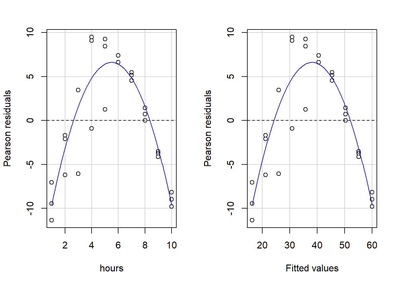

##            Test stat Pr(>|Test stat|)    
## hours        -11.466        6.988e-12 ***
## Tukey test   -11.466        < 2.2e-16 ***
## ---
## Signif. codes:  0 '***' 0.001 '**' 0.01 '*' 0.05 '.' 0.1 ' ' 1

When we visually inspect these plots, we see that the blue lines are not even close to straight, so key OLS assumptions are violated. And if we look at the written output, it is clear that we fail both a) the goodness of fit test for hours, the only independent variable, and b) the Tukey test for the overall model.

Clearly, we need to re-specify our regression model so that we can fit the data better and also so that we can avoid violating OLS regression assumptions. Keep reading to see how we can do that!

6.1.1.2 Inspecting the data

Above, we saw that running a linear regression the way we normally do does not fit our data well. But we don’t necessarily know how to fix the problem. A good first step is to visually inspect the relationship that we are trying to understand.

Let’s look at a scatterplot of the data to see what might be going on. Below is a plot with lift—our dependent variable of interest—and hours—our independent variable of interest—plotted against each other.

Here is the plot:

plot(mf$hours, mf$lift)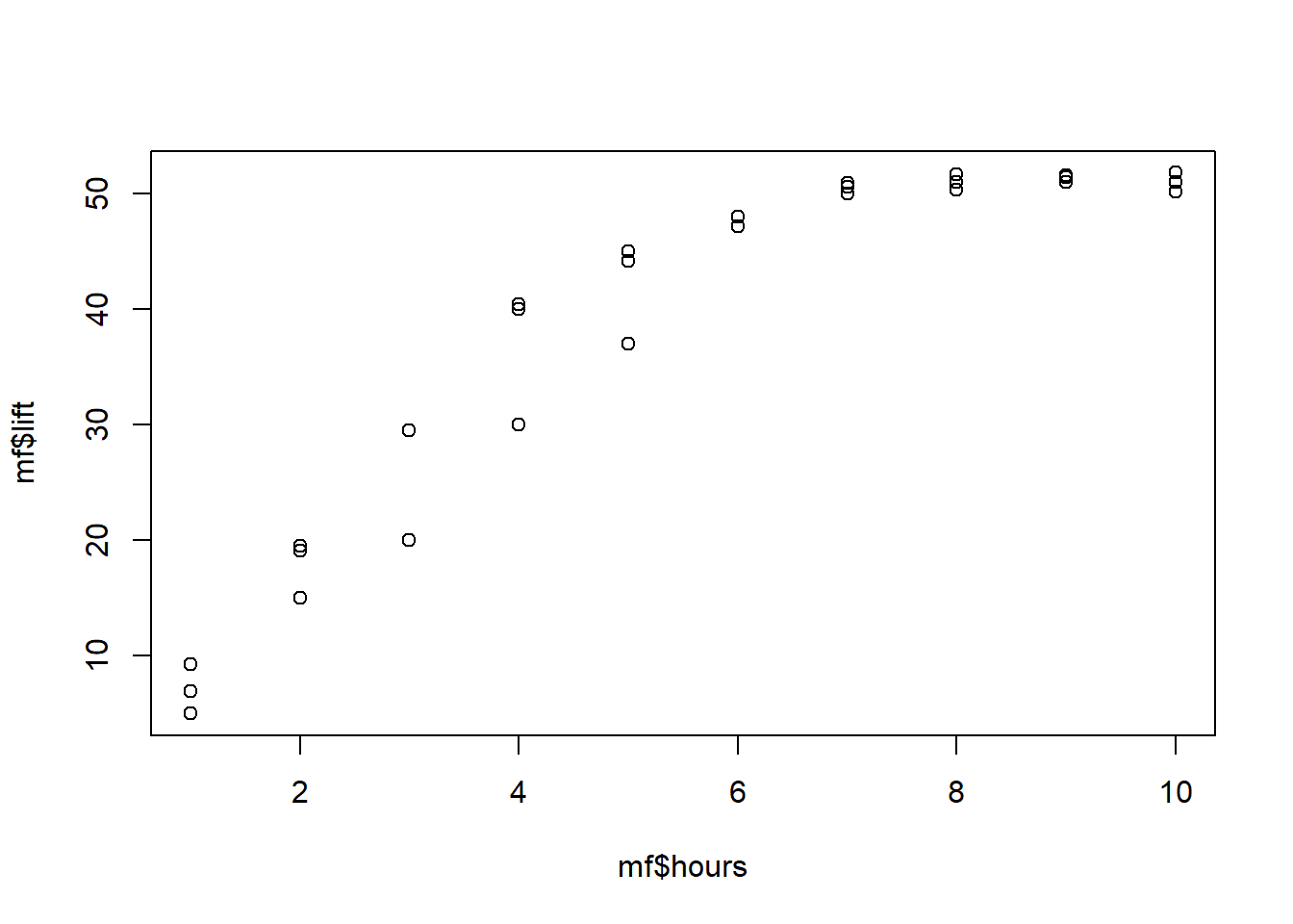

The data are not really in a straight line. The relationship starts off sort of linear—looking from lower to higher number of hours—but then seems to level off. Clearly, this is a non-linear trend, meaning that lift and hours do not vary linearly with one another. A straight line is not the best description of their relationship.

But linear regression only fits linear trends. We have to somehow tell the computer that it is free to fit a non-linear, or curvilinear trend to the data. To do this, we add a quadratic term as an independent variable in the model. A quadratic term just means a squared term.

As you may recall from math classes before, a polynomial equation that has an \(x^2\) term in it (and no \(x\) terms with higher exponents, like \(x^3\)), such as \(y = x^2\), will result in a parabola.

So our new goal is to fit not a line, but a parabola to our data.

Read on to see how to do this in R and how to interpret the results!

6.1.1.3 Preparing the data

To tell R that we want to fit a parabola rather than a line to our data, we will need to add a squared regression term to our regression formula in the lm() command. First, we need to create a squared version of the independent variable that we want to add to the model. In this case, that variable is hours.

Note that in the future you will likely have regression models with more than one independent variable. In that situation, you can add squared terms for some but not all of the independent variables into the model. (You can also add squared terms for all of the variables if you want). You do not need to add squared terms for all independent variables, only the ones that you suspect have a curvilinear/parabolic relationship with the dependent variable. We can come to suspect such a relationship by running diagnostic tests, by visually inspecting our data, or even by theorizing that it may be the case.

Here’s how we create the squared term:

mf$hoursSq <- mf$hours^2

The code above is saying the following:

• mf$hoursSq – Within the dataset mf, create a new variable called hoursSq.
• <- – The new variable to left will be assigned to the value generated by the code to the right.
• mf$hours^2 – Within the dataset mf, get the value of the variable hours for each observation and square it.

Now, let’s inspect the data once again:

mf

##         name lift hours hoursSq
## 1  Person 01  5.0     1       1
## 2  Person 02 15.0     2       4
## 3  Person 03 20.0     3       9
## 4  Person 04 30.0     4      16
## 5  Person 05 37.0     5      25
## 6  Person 06 48.0     6      36
## 7  Person 07 50.0     7      49
## 8  Person 08 51.0     8      64
## 9  Person 09 51.0     9      81
## 10 Person 10 51.0    10     100
## 11 Person 11  6.9     1       1
## 12 Person 12 19.5     2       4
## 13 Person 13 29.5     3       9
## 14 Person 14 40.4     4      16
## 15 Person 15 45.0     5      25
## 16 Person 16 48.0     6      36
## 17 Person 17 50.9     7      49
## 18 Person 18 50.3     8      64
## 19 Person 19 51.4     9      81
## 20 Person 20 51.8    10     100
## 21 Person 21  9.3     1       1
## 22 Person 22 19.1     2       4
## 23 Person 23 29.5     3       9
## 24 Person 24 40.0     4      16
## 25 Person 25 44.2     5      25
## 26 Person 26 47.2     6      36
## 27 Person 27 50.6     7      49
## 28 Person 28 51.7     8      64
## 29 Person 29 51.6     9      81
## 30 Person 30 50.2    10     100

You can see that a new column of data—called hoursSq—has been added for the new squared version of the independent variable hours. Keep in mind that R automatically squared the value of hours separately for us in each observation (each row) and then placed that new squared value in that same row in the new column for hoursSq. For example, see row #4. This person, labeled as Person 4, spends 4 hours lifting weights per week, which we can see in row #4 in the hours column. And then we can see that the computer has added the number 16 in the column hoursSq for Person 4.

Now that we have our new squared variable in the model, we can run another regression.

6.1.1.4 Running and interpreting quadratic regression

We are now ready to run our new regression with a quadratic (squared) term included as an independent variable. To do this, we use the same lm() command that we always do, but we include our newly created squared term—hoursSq—as an independent variable. It is important to note that even though we are now adding the hoursSq variable to our model, we still need to keep the un-squared hours variable in as well.

Here is the code to run the new regression:

summary(reg2 <- lm(lift ~  hours + hoursSq, data = mf))

## 
## Call:
## lm(formula = lift ~ hours + hoursSq, data = mf)
## 
## Residuals:
##     Min      1Q  Median      3Q     Max 
## -7.6556 -0.8003  0.2714  1.4855  4.6908 
## 
## Coefficients:
##             Estimate Std. Error t value Pr(>|t|)    
## (Intercept) -6.12500    1.88959  -3.241  0.00315 ** 
## hours       13.66513    0.78917  17.316 3.80e-16 ***
## hoursSq     -0.80164    0.06992 -11.466 6.99e-12 ***
## ---
## Signif. codes:  0 '***' 0.001 '**' 0.01 '*' 0.05 '.' 0.1 ' ' 1
## 
## Residual standard error: 2.783 on 27 degrees of freedom
## Multiple R-squared:  0.9703, Adjusted R-squared:  0.9681 
## F-statistic: 441.2 on 2 and 27 DF,  p-value: < 2.2e-16

One of the first numbers that should pop out at you is the extremely high \(R^2\) statistic. This indicates that the new regression model fits the data extremely well.¹¹⁸ The variation in the independent variables explains over 90% of the variation in the dependent variable!

Keep in mind that we did not add any new data to the model. All we did is tell the computer to look for a curved, parabolic trend, rather than solely a linear trend. Doing this allowed us to create a regression model that fit our data much better than before.

The equation for this new quadratic regression result is:

\[\hat{lift} = -6.13 + 13.67*hours -0.8*hours^2\]

If we rewrite this in terms of just Y and X, it looks like this:

\[\hat{y} = -6.13 + 13.67x -0.8x^2\]

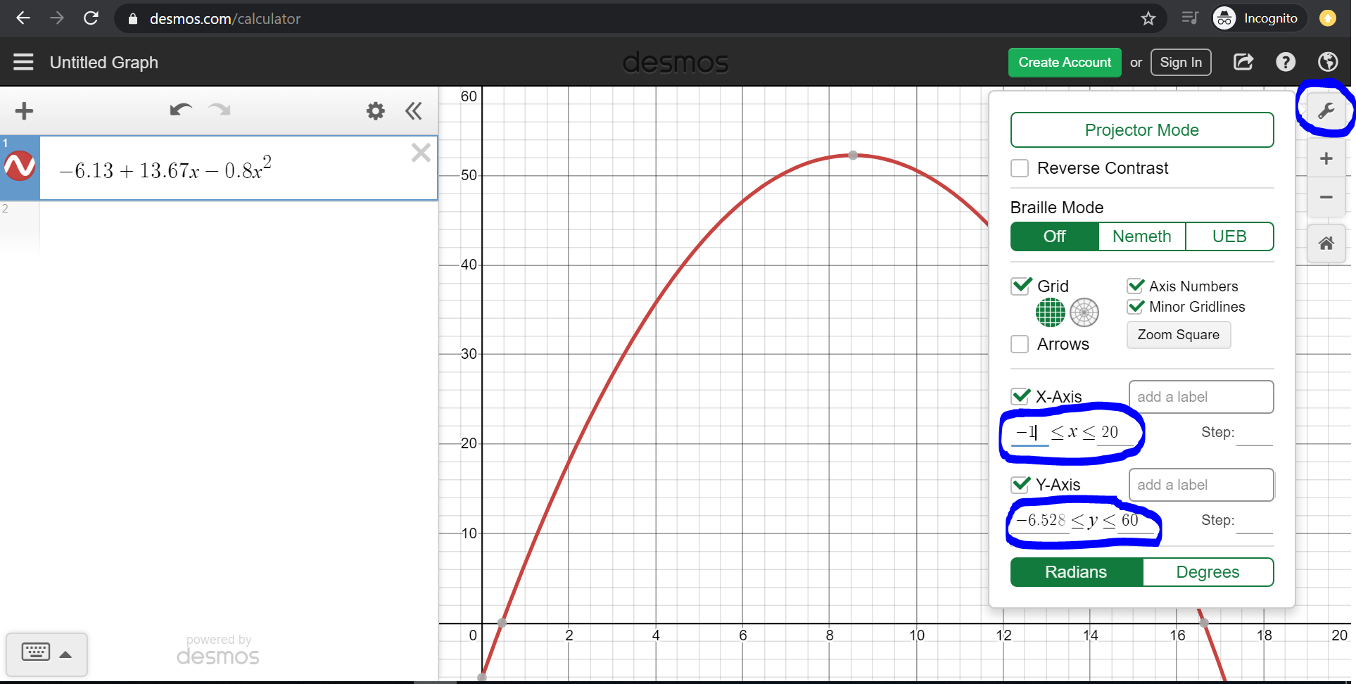
This is the equation of the parabola that fits our data. Let’s plot this equation into a graphing calculator. Click here to open a graphing calculator. Copy and paste (or retype) the following into the graphing calculator:

-6.13 + 13.67x -0.8x^2

Next, change the axes by clicking on the wrench in the top-right corner, so that the parabola is framed well.

Please follow these steps and see the screenshot below:

1. Paste -6.13 + 13.67x -0.8x^2 into the equation box in the top-left corner.
2. Click on the wrench in the top-right corner which is circled in blue.
3. Change the x-axis to range from approximately -1 to 20 in the bottom right, where the blue circle is.
4. Change the y-axis to range from approximately -5 to 60 in the bottom right, where the blue circle is.

Then you should see the entire portion of the parabola that is in the range of our data.

We can also plot this in R, along with our data points:¹¹⁹

eq2 = function(x){-6.13 + 13.67*x -0.8*(x^2)}

if (!require(ggplot2)) install.packages('ggplot2')

## Warning: package 'ggplot2' was built under R version 4.2.3

library(ggplot2)

ggplot(data.frame(x=c(1, 14)), aes(x=x)) + stat_function(fun=eq2) + geom_point(aes(x=hours, y=lift), data = mf)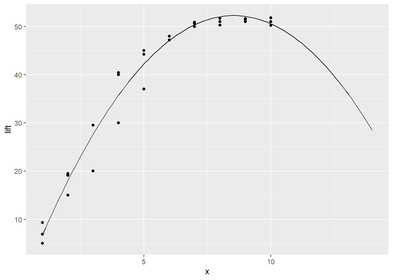

Our new model seems to fit the data pretty well, and it captures the nonlinear nature of the relationship between lift and hours.

This result tells us that weight lifting capability increases as weekly weightlifting hours go up, until we reach about 7 hours per week of weightlifting. The slope is steep at first (at lower levels of hours on the x-axis) but then it levels off and becomes less steep. This is basically suggesting that the gains or returns to weightlifting level off as you train more.

Note that we do not interpret hours and hoursSq separately. hours and hoursSq are two versions of the same data and they are both helping us determine the relationship between weight lifting capability and weekly weightlifting hours.

Such a trend is sometimes referred to as decreasing/diminishing marginal returns. The slope becomes less and less positive at higher values of the independent variable. In other words, the added benefit of each additional hour of weightlifting is predicted to be less and less as you weightlift more.

For people who do more than about 10 hours per week, the model is actually predicting a decrease in weightlifting capability with each increased hour of weight training. This prediction is probably incorrect. So we have to remember that even though this model fits our data much better, it also makes predictions that might not always make sense when we look at the extreme ends of our data range.

Note that we left the unsquared hours variable in the model, in addition to the hoursSq variable. It is essential to leave the unsquared variable in the model as well. Do not remove it! Also note that this is still OLS linear regression, even though we used it to fit a non-linear trend.

6.1.1.5 Residual plots for quadratic regression

Above, we ran a quadratic regression and it appears that we were able to fit our regression model to the data quite well. But the very next thing we should always do is to look at the residual plots of the new regression model.

Here they are:

residualPlots(reg2)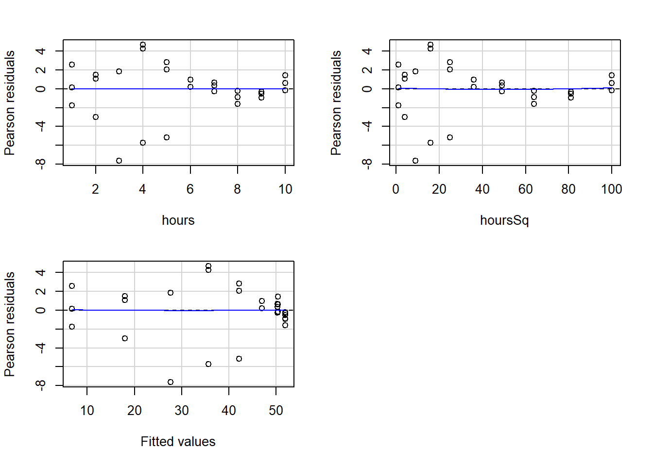

##            Test stat Pr(>|Test stat|)   
## hours         2.9829         0.006135 **
## hoursSq       0.2386         0.813257   
## Tukey test    0.0515         0.958897   
## ---
## Signif. codes:  0 '***' 0.001 '**' 0.01 '*' 0.05 '.' 0.1 ' ' 1

As you may recall from earlier in the chapter, when we did not have a squared term in the regression, our residuals appeared to be correlated with the independent variable hours as well as with the fitted values of the regression.

Now look again at the new residual plots above. They look much better and are no longer violating the tested regression assumptions! The blue lines are straight, horizontal, and hugging the horizontal line in the charts.

Remember, in this example, above we only ran the residual plots diagnostics. However, when you use OLS linear regression for real research, instead of practice like this, you have to test all of the OLS regression assumptions, just like you practiced in a previous assignment. Before testing these assumptions, you cannot fully trust the results you see in the regression output summary!

6.1.2 Other transformations – optional

Reading this section is completely optional and not required.

The squared/quadratic transformation that we examined in detail above is not the only way to transform your data. The quadratic transformation is only to fit a parabola to your data. If you notice that the relationship you want to study is non-linear but likely does not follow a parabolic trajectory, there are other transformations that you can try. We will not look at these other transformations much or at all in this course, but it is important to be aware that other options exist.

Log transformations are one of the most commonly used transformations to improve the fit of regression models to data.

Here are some resources related to log and other transformations:

• Interpreting Log Transformations in a Linear Model
• Chapter 14 “Transformations” in Applied Statistics with R.
• Transformations of Variables – This resource features a nice table that compares many types of transformations to each other.

Once again, reading these resources about other types of transformations is completely optional (not required).

6.2 Interactions

Previously, we learned how to use dummy variables to model regression equations for different groups within our data. In these situations, we created multiple parallel estimates for each group of observations according to the dummy variable. For example, we drew two parallel regression lines to show predictions for two different groups of people. In this situation, the association (slope) between the dependent and independent variable(s) was the same for everyone, and intercept was different for observations in each level of the dummy variable.

Now we will explore another possibility: What if the association (slope) between the dependent variable and independent itself is different for different groups of observations in our data? To investigate this, we will use what we call interaction.

In this section, we will go through how to interact two independent variables with each other. We will interact dummy variables with continuous numeric variables and add this interaction to a regression model.

There are two videos below that you can decide if you want to watch before or after reading the text.

The first video introduces the concept of interaction effects and demonstrates a few common ways to visualize them:

The video above can also be viewed externally at https://youtu.be/UzZozpxatWQ.

The second video shows selected key details and concepts related to interactions in regression analysis, as a supplement to the text:

The video above can also be viewed externally at https://youtu.be/9lQW7B5YpLk.

6.2.1 Review of no-interaction example

We will begin by briefly reviewing what we already know from before: how to make an OLS model with separate continuous and dummy variables.

Throughout this part of the chapter, we will use some example data—called d—in which each observation is a person. We will answer the following question: What is the association between outcome and age?

Our data initially includes the following variables:

• Outcome – This is our outcome of interest. It is a continuous numeric variable. We don’t know any more details than that about what this outcome is measuring or if this outcome is something that is good or bad.
• Age – Age of the person in years. This is a continuous numeric variable.
• Gender – Gender category of the person. This is a qualitative categorical variable.

Let’s load the data by running the following code:

outcome <- c(0.5, 2.45, 0.92, 4.9, 5.53, 4.62, 6.88, 6.59, 9.82, 8.68, 4.25, 5.5, 3.31, 5.78, 6.31, 3.21, 5.37, 6.64, 7.69, 5.18)

age <- c(1,2,3,4,5,6,7,8,9,10,1,2,3,4,5,6,7,8,9,10)


gender <- c(rep("female",10),rep("male",10))

d <- data.frame(outcome, age, gender)

Now we have a dataset containing 10 females and 10 males loaded into R as d, shown below:

d

##    outcome age gender
## 1     0.50   1 female
## 2     2.45   2 female
## 3     0.92   3 female
## 4     4.90   4 female
## 5     5.53   5 female
## 6     4.62   6 female
## 7     6.88   7 female
## 8     6.59   8 female
## 9     9.82   9 female
## 10    8.68  10 female
## 11    4.25   1   male
## 12    5.50   2   male
## 13    3.31   3   male
## 14    5.78   4   male
## 15    6.31   5   male
## 16    3.21   6   male
## 17    5.37   7   male
## 18    6.64   8   male
## 19    7.69   9   male
## 20    5.18  10   male

Next, we need to recode the variable gender into a dummy variable:

d$female <- ifelse(d$gender=="female",1,0)

Above, we created a new dummy variable called female which is coded as 1 for females and 0 for males.

Here is what the dataset looks like now:

d

##    outcome age gender female
## 1     0.50   1 female      1
## 2     2.45   2 female      1
## 3     0.92   3 female      1
## 4     4.90   4 female      1
## 5     5.53   5 female      1
## 6     4.62   6 female      1
## 7     6.88   7 female      1
## 8     6.59   8 female      1
## 9     9.82   9 female      1
## 10    8.68  10 female      1
## 11    4.25   1   male      0
## 12    5.50   2   male      0
## 13    3.31   3   male      0
## 14    5.78   4   male      0
## 15    6.31   5   male      0
## 16    3.21   6   male      0
## 17    5.37   7   male      0
## 18    6.64   8   male      0
## 19    7.69   9   male      0
## 20    5.18  10   male      0

In our data above, we will ignore the original categorical variable gender and we will only use our new dummy variable female. Remember: the computer can only use numbers; it cannot handle the concept of gender unless we trick it by converting into 1 and 0.

We are ready to run OLS on our data using now-familiar code:

ols1 <- lm(outcome ~ age+female, data = d)

if (!require(jtools)) install.packages('jtools')
library(jtools)
summ(ols1, confint = TRUE)

Observations	20
Dependent variable	outcome
Type	OLS linear regression

F(2,17)	10.33
R²	0.55
Adj. R²	0.50

	Est.	2.5%	97.5%	t val.	p
(Intercept)	2.08	0.20	3.96	2.34	0.03
age	0.59	0.32	0.86	4.53	0.00
female	-0.23	-1.81	1.34	-0.31	0.76
Standard errors: OLS

Above, we see in our new OLS model—called ols1—that in our sample, the outcome increases by 0.59 units on average for each one year increase in age, controlling for gender. We also see that in our sample, females are predicted to have an outcome that is 0.23 units lower than the outcome of males on average, controlling for age.

We can visualize this outcome as we have before with the interact_plot(...) function:

if (!require(interactions)) install.packages('interactions')
library(interactions)

interact_plot(ols1, pred = age, modx = female, plot.points = TRUE)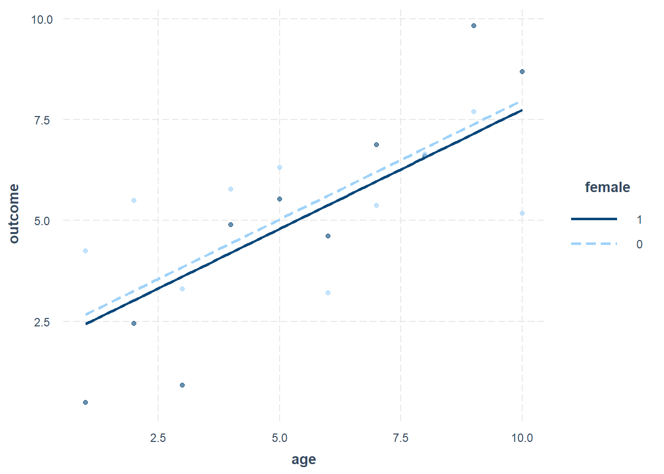

Note that details about how to make an interaction plot for yourself are provided later in this chapter.

This regression model enabled us to answer these questions of interest:

1. What is the average relationship between outcome and age, controlling for all other independent variables?¹²⁰ Answer: 0.59 units average increase in outcome per additional year of age.
2. What is the average difference in outcome between men and women, controlling for all other independent variables?¹²¹ Answer: females are 0.23 units lower than males on average.

Above, we see a minor difference in intercepts between females (coded as 1) and males (coded as 0). The slope of outcome against age is of course the same for both genders. This was a replication of the method you already knew from before, in which we use OLS to examine the relationship between a continuous dependent variable (outcome) and continuous independent variable (age) separately for two groups.

6.2.2 Two-category interaction

Let’s turn to a new and related question: What is the association between outcome and age, separately for females and males?

Earlier, we made separate regression lines for females and males, and each of these lines had the same slope as each other. Now we want to investigate if this slope could actually be different for males and females in our sample. To do this, we have to add to our OLS model what is called an interaction term. An interaction term is created by adding an additional independent variable to our OLS model. This new variable is just the multiplication of the two variables that we want to interact with each other, typically one continuous numeric variable and one dummy numeric variable. The process is demonstrated below.

6.2.2.1 Run OLS model with interaction in R

In the current example, we want to interact age and female. We will do this by creating a new variable which is the result of multiplying age and female with each other.

The code below creates our new interaction variable:

d$age.female <- d$age * d$female

Here is what the code above asked the computer to do:

• d$age.female <- – Create a new variable called age.female within the dataset d. Each observation’s value of this new variable will be assigned by the code that follows the <- operator.
• d$age * d$female – For each observation within the dataset d, multiply age and female.

We can inspect our data, which now includes the new variable age.female:

d

##    outcome age gender female age.female
## 1     0.50   1 female      1          1
## 2     2.45   2 female      1          2
## 3     0.92   3 female      1          3
## 4     4.90   4 female      1          4
## 5     5.53   5 female      1          5
## 6     4.62   6 female      1          6
## 7     6.88   7 female      1          7
## 8     6.59   8 female      1          8
## 9     9.82   9 female      1          9
## 10    8.68  10 female      1         10
## 11    4.25   1   male      0          0
## 12    5.50   2   male      0          0
## 13    3.31   3   male      0          0
## 14    5.78   4   male      0          0
## 15    6.31   5   male      0          0
## 16    3.21   6   male      0          0
## 17    5.37   7   male      0          0
## 18    6.64   8   male      0          0
## 19    7.69   9   male      0          0
## 20    5.18  10   male      0          0

Let’s consider two examples from the data spreadsheet above:

• The third observation, in the third row, is a female. Her age is 3 and her female variable is 1. So her age.female is the multiplication of 3 and 1, which is 3.
• The final observation, in the 20th and final row, is a male. His age is 10 and his female variable is 0. So his age.female variable is 0, which is the result of multiplying 10 and 0.

It looks like our new variable was generated correctly! Now we can run a new OLS model in which we include the new variable age.female as an additional independent variable. Note that we still must include age and female in the model as well; we cannot remove them.

Here we run our new model, which we save as ols2:¹²²

ols2 <- lm(outcome ~ age + female + age.female, data = d)

And now we can create a results table:

if (!require(jtools)) install.packages('jtools')
library(jtools)

summ(ols2, confint = TRUE)

Observations	20
Dependent variable	outcome
Type	OLS linear regression

F(3,16)	17.37
R²	0.77
Adj. R²	0.72

	Est.	2.5%	97.5%	t val.	p
(Intercept)	4.12	2.32	5.92	4.86	0.00
age	0.22	-0.07	0.51	1.60	0.13
female	-4.32	-6.86	-1.78	-3.60	0.00
age.female	0.74	0.33	1.15	3.84	0.00
Standard errors: OLS

Before we carefully interpret the results above, let’s first visualize these results, such that our eventual interpretation is more intuitive.

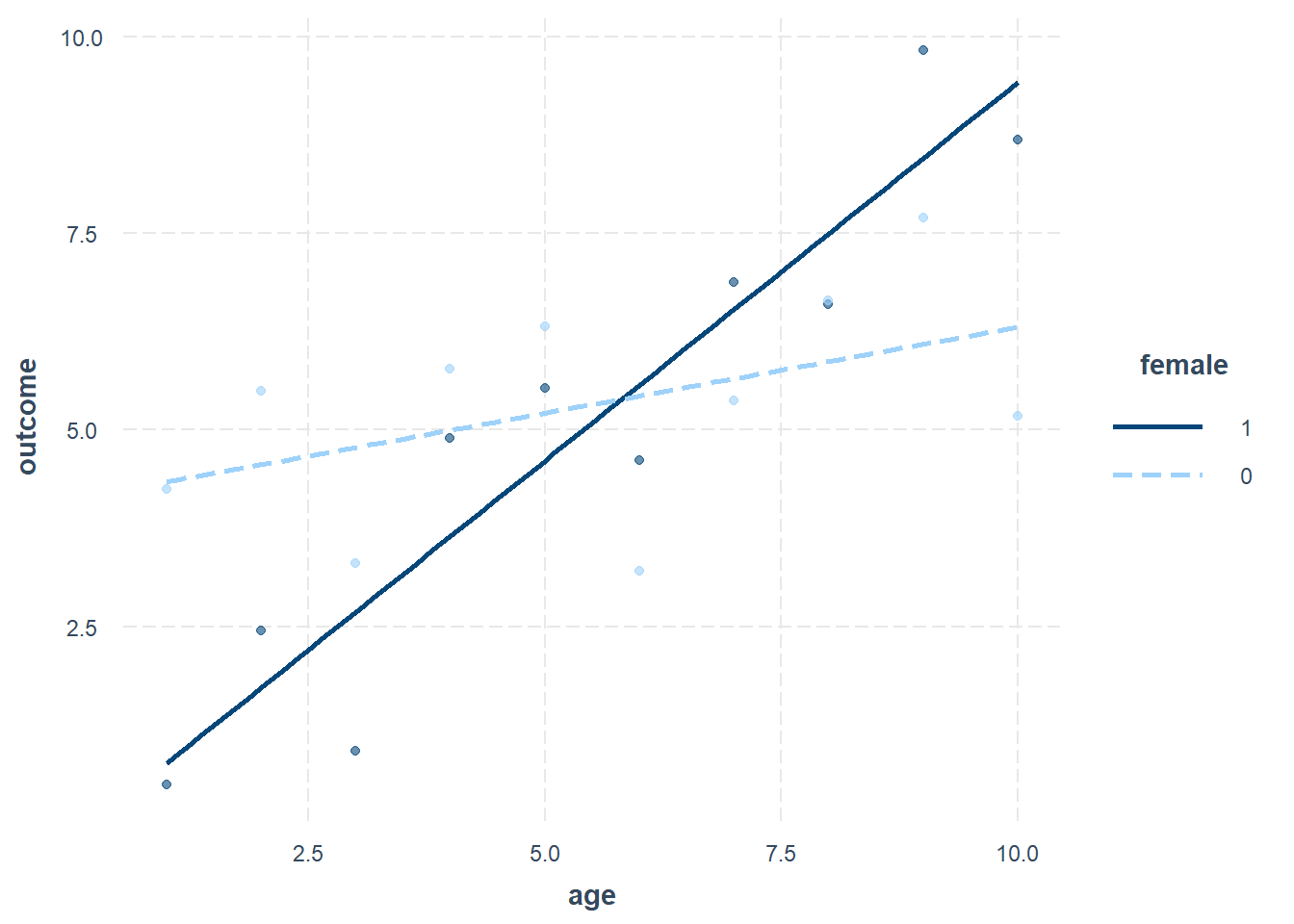
Here is a plot showing our ols2 regression result:

We will learn how to make a plot like this later in this chapter.

This regression model enabled us to answer these questions of interest:

1. What is the average relationship between outcome and age only for males? Answer: 0.22 units average increase in outcome per additional year of age.
2. What is the average relationship between outcome and age only for females? Answer: 0.96 units average increase in outcome per additional year of age.¹²³

The plot above shows the interaction of the independent variables age and female. The interaction occurs between independent variables only. The addition of this interaction then helps us answer our question of interest, which is: What is the association between outcome and age, separately for females and males? In the plot, we see separate lines for males and females! We successfully visualized the association between outcome and age separately for each gender.

Remember: The whole reason we are using an interaction is to discover the two separate lines shown in the plot above. We see that the relationship between outcome and age in our sample is different for each gender group, because the lines have different slopes.

Let’s make some qualitative observations of our plotted result, without using numbers:

• The two lines in the plot clearly have different slopes.
• For both genders, as age increases, outcome is also predicted to increase on average in our sample.
• However, this predicted increase in outcome happens at a different rate (slope) for females and males.
• The plot also tells us that on average in our sample: females under the age of six years are lower than males under the age of six years on outcome, while females over the age of six years are higher than males over the age of six years on outcome. Note that six years is approximately where the two lines cross.

6.2.2.2 Sample interpretation of OLS with two-category interaction

Now it’s time to fully interpret our regression results, copied again here:

Observations	20
Dependent variable	outcome
Type	OLS linear regression

F(3,16)	17.37
R²	0.77
Adj. R²	0.72

	Est.	2.5%	97.5%	t val.	p
(Intercept)	4.12	2.32	5.92	4.86	0.00
age	0.22	-0.07	0.51	1.60	0.13
female	-4.32	-6.86	-1.78	-3.60	0.00
age.female	0.74	0.33	1.15	3.84	0.00
Standard errors: OLS

As we always do, we will first interpret regression results for our sample before moving on to using inference to interpret results for our population.

Let’s begin by writing the equation for this OLS model, in a few different ways:

1. This is how the equation looks if we take it directly from the regression table: \(\hat{outcome} = 0.22age - 4.32female + 0.74age.female + 4.12\)
2. Another way to write this equation is this, with multiplication signs included: \(\hat{outcome} = 0.22*age - 4.32*female + 0.74*age.female + 4.12\). This just reminds us that we are multiplying each slope by each variable in the equation.
3. We know that the variable age.female is actually the multiplication of age and female, so let’s rewrite the equation to reflect that: \(\hat{outcome} = 0.22*age - 4.32*female + 0.74*age*female + 4.12\). This is our final equation.

Our final equation is:

\[\hat{outcome} = 0.22*age - 4.32*female + 0.74*age*female + 4.12\]

Now it’s time to make separate equations for females and males. Remember, the variable female is coded as 1 for females and 0 for males. We are going to plug in these numbers for female to create separate equations. The procedure for doing this is shown below for females and males one at a time.

Unique equation for females:

1. Start with complete regression equation from earlier: \(\hat{outcome} = 0.22*age - 4.32*female + 0.74*age*female + 4.12\)
2. Plug in 1 for female variable: \(\hat{outcome}_{female} = 0.22*age - 4.32*1 + 0.74*age*1 + 4.12\)
3. Move terms¹²⁴ around: \(\hat{outcome}_{female} = 0.22*age + 0.74*age*1 - 4.32*1 + 4.12\)
4. Start to combine terms: \(\hat{outcome}_{female} = (0.22 + 0.74)*age + (-4.32*1 + 4.12)\)
5. Finish combining terms: \(\hat{outcome}_{female} = 0.96*age - 0.2\)

Unique equation for males:

1. Start with complete regression equation from earlier: \(\hat{outcome} = 0.22*age - 4.32*female + 0.74*age*female + 4.12\)
2. Plug in 0 for female variable: \(\hat{outcome}_{male} = 0.22*age - 4.32*0 + 0.74*age*0 + 4.12\)
3. Eliminate terms that are multiplied by 0: \(\hat{outcome} = 0.22*age + 4.12\)

These are the final equations for each group and their interpretations:

• Females: \(\hat{outcome}_{female} = 0.96*age - 0.2\)
  • Slope of age: For each additional year of age, females in our sample are predicted to have an additional 0.96 units of outcome.
  • Intercept: The average predicted outcome for a female in our sample who is 0 years old is -0.2 units.
• Males: \(\hat{outcome}_{male} = 0.22*age + 4.12\)
  • Slope of age: For each additional year of age, males in our sample are predicted to have an additional 0.22 units of outcome.
  • Intercept: The average predicted outcome for a male in our sample who is 0 years old is 4.12 units.

Above, we simply interpreted the regression equations for females and males as if they were a regular regression equation that had not been generated from interactions. We split our samples into two groups—female and male—and created a separate equation for each group. In this case, the two groups were the two different values of our female variable.

Here are a few other key details about our regression result and the final equations we calculated (the details below are just a review of the results above, approach in a different way):

• Slope of outcome and age:
  • The slope of age for females is 0.96.
  • The slope of age for males is 0.22.
  • The difference between these two slopes is \(0.96 - 0.22 = 0.74\).
  • Now look at the regression results table again.
  • 0.22 is the slope for the age variable in the table.
  • 0.74 is the slope for the age.female variable in the table.
  • This means that 0.22 is the slope of the association between outcome and age for observations that have age.female as 0, which is the case only for males.
  • 0.74 is the addition to the slope of 0.22 for observations that have age.female as 1, which is the case only for females.
  • Therefore, \(0.22 + 0.74 = 0.96\) gives us the slope of the association between outcome and age for females.
• Intercept:
  • The intercept for females is -0.2.
  • The intercept for males is 4.12.
  • The difference between these two intercepts is \(-0.22-4.12 = -4.32\).
  • Now look at the regression results table again.
  • The intercept of the model is 4.12.
  • The slope for the female variable is -4.32.
  • This means that 4.12 is the intercept in this regression model for observations that have female as 0, which is the case only for males.
  • -4.32 is the addition to the intercept of 4.12 for observations that have female as 1, which is the case only for females.
  • Therefore, \(4.12 - 4.32 = 0.2\) gives us the intercept for females.

6.2.2.3 Population interpretation of OLS with interaction

Now that we have fully explored our OLS results as they pertain to the sample, we can do the same for the population. We will do this in a slightly more abbreviated fashion. As we do this, we will keep the regression equations for females and males in mind, but we will not write more equations. Instead, we will calculate 95% confidence intervals of the slope and intercept in the population separately for females and males.

Below, we walk through the process separately for each item we want to calculate in the population:

1. Population slope of outcome and age for females only
   1. Remember that this slope estimate for females is calculated by adding the slopes of age and age.female to each other. Now we just need to do this adding process for the lower and upper confidence interval bounds.
   2. Lower bound: age is -0.07. age.female is 0.33. When we add these numbers together we get 0.26.
   3. Upper bound: age is 0.51. age.female is 1.15. When we add these numbers together we get 1.66.
   4. Therefore: We are 95% confident that for each one year increase in age, outcome is predicted to increase by at least 0.33 units and at most 1.66 units on average for the female members of our population.
2. Population slope of outcome and age for males only
   1. Remember that this slope estimate for males is just the estimate for age. All we need to do is look at the lower and upper confidence interval bounds of age.
   2. Lower bound: age is -0.07.
   3. Upper bound: age is 0.51.
   4. Therefore: We are 95% confident that for each one year increase in age, outcome is predicted to increase by at least -0.07¹²⁵ units and at most 0.51 units on average for the male members of our population.
3. Population intercept of outcome for females only
   1. Remember that this intercept estimate for females is calculated by adding the intercept and the female estimates to each other. Now we just need to repeat this process for the lower and upper confidence interval bounds.
   2. Lower bound: intercept is 2.32. female is -6.86. When we add these numbers together we get -4.54.
   3. Upper bound: intercept is 5.92. female is -1.78. When we add these numbers together we get 4.14.
   4. Therefore: We are 95% confident that when age is 0, the predicted value of outcome is at least -4.54 units and at most 4.14 units on average for the female members of our population.
4. Population intercept of outcome for males only
   1. Remember that this intercept estimate for males is just the estimate of the intercept in the regression model. All we need to do is look at its lower and upper confidence interval bounds.
   2. Lower bound: 2.32.
   3. Upper bound: 5.92.
   4. Therefore: We are 95% confident that when age is 0, the predicted value of outcome is at least 2.32 units and at most 5.92 units on average for the male members of our population.

Of course, before we can trust these results for inference (meaning for the population of interest rather than just our sample), we would have to run all OLS diagnostic tests that you have learned about before and all of the tests would have to pass.

6.2.3 Three-category interaction

In this section, we will repeat the process that we learned above (a two-category interaction) but now for a three-category interaction. Remember, the question we are trying to answer is still: What is the association between outcome and age , separately for each gender? This time, we will add a third gender to the data.

Let’s run the following code to recreate our data, this time including a gender called nonbinary:

outcome <- c(0.5, 2.45, 0.92, 4.9, 5.53, 4.62, 6.88, 6.59, 9.82, 8.68, 4.25, 5.5, 3.31, 5.78, 6.31, 3.21, 5.37, 6.64, 7.69, 5.18, 3,4,3,4,3,4,3,4,3,4)

age <- c(1,2,3,4,5,6,7,8,9,10,1,2,3,4,5,6,7,8,9,10,1,2,3,4,5,6,7,8,9,10)

gender <- c(rep("female",10),rep("male",10), rep("nonbinary",10))

d2 <- data.frame(outcome, age, gender)

We have now created a new dataset called d2 with 30 observations, containing ten female, ten male, and ten nonbinary people. We also have outcome and age measures for each observation (which in this case is a person). This is the same as the dataset d that we used above, now with ten observations added compared to before.

6.2.3.1 Run OLS model with three-category interaction in R

The next step we need to repeat on our new data is that we need to create dummy variables for each category of the variable gender. We can do this using the fastDummies package, as we have done before.

Here we create the new gender dummy variables:

if (!require(fastDummies)) install.packages('fastDummies')
library(fastDummies)

d2 <- dummy_cols(d2,select_columns = c("gender"))

After running the code above, three new variables have been added to our dataset d2. If you are following along, you can run the command View(d2) or names(d2) to confirm this.

Next—like before—we need to create interaction terms by using multiplication. We will do this for each of the dummy variables, to interact age with the three new dummy variables gender_female, gender_male, and gender_nonbinary.

This code creates the interaction terms:

d2$age.female <- d2$age * d2$gender_female
d2$age.male <- d2$age * d2$gender_male
d2$age.nonbinary <- d2$age * d2$gender_nonbinary

Now we can have a look at our data to make sure it is correct:

d2

##    outcome age    gender gender_female gender_male gender_nonbinary age.female
## 1     0.50   1    female             1           0                0          1
## 2     2.45   2    female             1           0                0          2
## 3     0.92   3    female             1           0                0          3
## 4     4.90   4    female             1           0                0          4
## 5     5.53   5    female             1           0                0          5
## 6     4.62   6    female             1           0                0          6
## 7     6.88   7    female             1           0                0          7
## 8     6.59   8    female             1           0                0          8
## 9     9.82   9    female             1           0                0          9
## 10    8.68  10    female             1           0                0         10
## 11    4.25   1      male             0           1                0          0
## 12    5.50   2      male             0           1                0          0
## 13    3.31   3      male             0           1                0          0
## 14    5.78   4      male             0           1                0          0
## 15    6.31   5      male             0           1                0          0
## 16    3.21   6      male             0           1                0          0
## 17    5.37   7      male             0           1                0          0
## 18    6.64   8      male             0           1                0          0
## 19    7.69   9      male             0           1                0          0
## 20    5.18  10      male             0           1                0          0
## 21    3.00   1 nonbinary             0           0                1          0
## 22    4.00   2 nonbinary             0           0                1          0
## 23    3.00   3 nonbinary             0           0                1          0
## 24    4.00   4 nonbinary             0           0                1          0
## 25    3.00   5 nonbinary             0           0                1          0
## 26    4.00   6 nonbinary             0           0                1          0
## 27    3.00   7 nonbinary             0           0                1          0
## 28    4.00   8 nonbinary             0           0                1          0
## 29    3.00   9 nonbinary             0           0                1          0
## 30    4.00  10 nonbinary             0           0                1          0
##    age.male age.nonbinary
## 1         0             0
## 2         0             0
## 3         0             0
## 4         0             0
## 5         0             0
## 6         0             0
## 7         0             0
## 8         0             0
## 9         0             0
## 10        0             0
## 11        1             0
## 12        2             0
## 13        3             0
## 14        4             0
## 15        5             0
## 16        6             0
## 17        7             0
## 18        8             0
## 19        9             0
## 20       10             0
## 21        0             1
## 22        0             2
## 23        0             3
## 24        0             4
## 25        0             5
## 26        0             6
## 27        0             7
## 28        0             8
## 29        0             9
## 30        0            10

Above, we see three new variables called age.female, age.male, and age.nonbinary Each one is the multiplication of an observation’s age and their dummy variable for each gender.

Now it is time to run our OLS regression in which we will interact the continuous numeric variable age with the dummy variables of the three-category categorical variable gender. When we do this—as is always the case when using dummy variables as independent variables in a regression model—we must leave one category out of the regression model. This time, we will leave out females and include males and nonbinary people. Females in this regression are the reference category because they are left out. This means that we will compare the results of males and nonbinary to females when we are interpreting our regression equation.

The code to run this OLS regression is below. Please note the following about this code:

• outcome is once again our dependent variable.
• age is a continuous numeric variable and we are including it on its own as usual.
• We include the non-interacted dummy variables for each non-reference gender category. This means that we include gender_male and gender_nonbinary, leaving out gender_female
• We include the interaction terms—meaning the interaction variables—that interact age with the non-reference gender categories. This means that we include age.male and age.nonbinary, leaving out age.female.
• We will call our regression model olsA below.

olsA <- lm(outcome ~ age + gender_male + gender_nonbinary + age.male  + age.nonbinary, data = d2)

if (!require(jtools)) install.packages('jtools')
library(jtools)

summ(olsA, confint = TRUE)

Observations	30
Dependent variable	outcome
Type	OLS linear regression

F(5,24)	17.69
R²	0.79
Adj. R²	0.74

	Est.	2.5%	97.5%	t val.	p
(Intercept)	-0.20	-1.70	1.30	-0.27	0.79
age	0.96	0.72	1.20	8.21	0.00
gender_male	4.32	2.20	6.44	4.21	0.00
gender_nonbinary	3.53	1.41	5.65	3.44	0.00
age.male	-0.74	-1.08	-0.40	-4.49	0.00
age.nonbinary	-0.93	-1.27	-0.59	-5.62	0.00
Standard errors: OLS

Before we carefully interpret the results above, let’s visualize these results, such that our eventual interpretation is more intuitive.

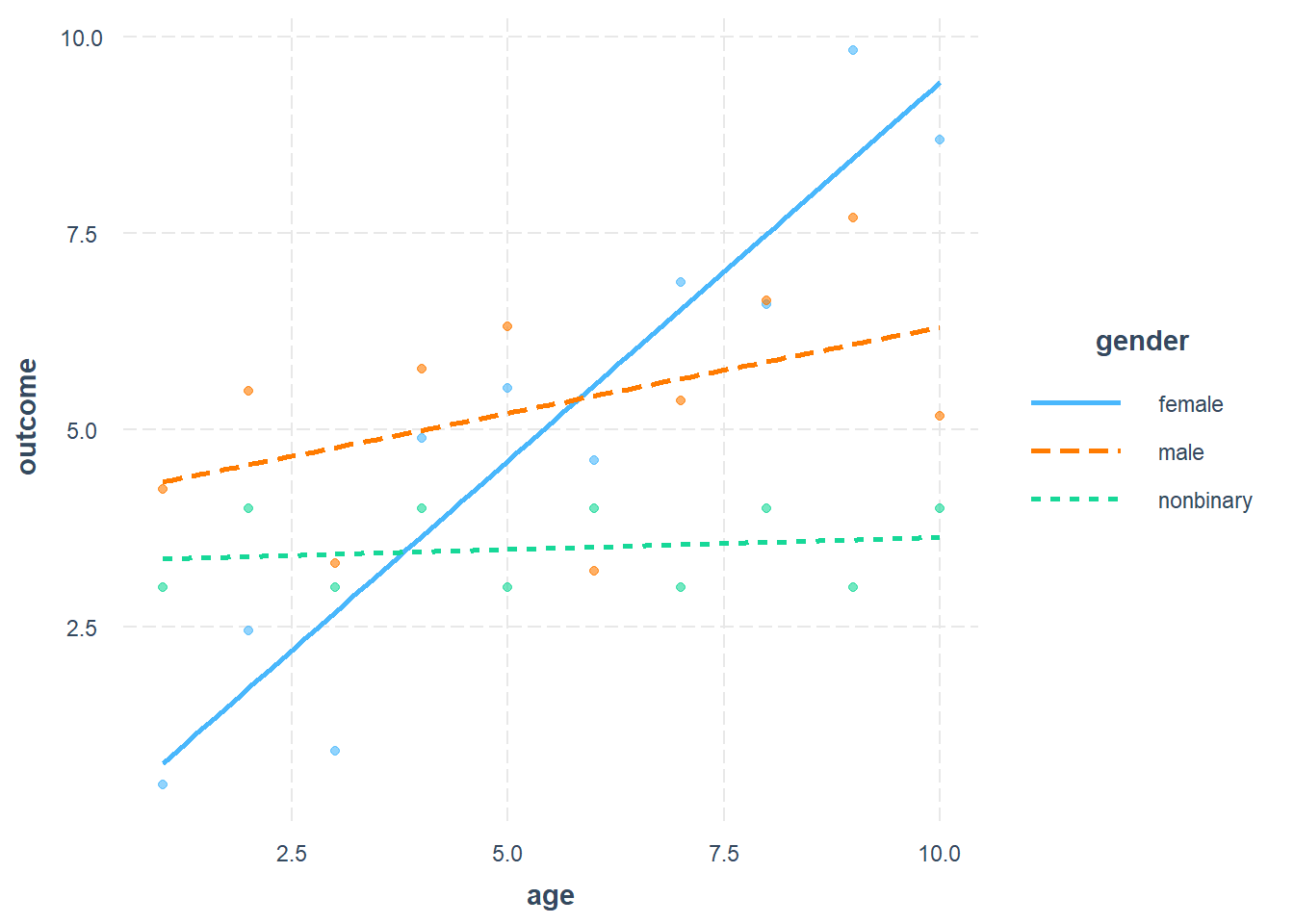
Here is a plot showing our olsA regression result:

Note that details about how to make an interaction plot for yourself are provided later in this chapter.

This regression model enabled us to answer these questions of interest:

1. What is the average relationship between outcome and age only for females? Answer: 0.96 units average increase in outcome per additional year of age.
2. What is the average relationship between outcome and age only for males? Answer: 0.22 units average increase in outcome per additional year of age.¹²⁶
3. What is the average relationship between outcome and age only for nonbinary people? Answer: 0.03 units average increase in outcome per additional year of age.¹²⁷

Above, we see the results of outcome regressed against age, separately for our three categories of gender.

Remember: The whole reason we are using an interaction is to discover the three separate lines shown in the plot above. We see that the relationship between outcome and age in our sample is different for each gender group, because the lines have different slopes.

Let’s again make some qualitative observations of our plotted result, without using numbers:

• For females: as age increases, outcome is predicted to increase quite a lot.
• For males: as age increases, outcome is predicted to increase a little bit.
• For nonbinary people: as age increases, outcome is predicted to increase very very little but basically not at all.

6.2.3.2 Sample interpretation of OLS with three-category interaction

Now it’s time to fully interpret our regression results, copied again here:

Observations	30
Dependent variable	outcome
Type	OLS linear regression

F(5,24)	17.69
R²	0.79
Adj. R²	0.74

	Est.	2.5%	97.5%	t val.	p
(Intercept)	-0.20	-1.70	1.30	-0.27	0.79
age	0.96	0.72	1.20	8.21	0.00
gender_male	4.32	2.20	6.44	4.21	0.00
gender_nonbinary	3.53	1.41	5.65	3.44	0.00
age.male	-0.74	-1.08	-0.40	-4.49	0.00
age.nonbinary	-0.93	-1.27	-0.59	-5.62	0.00
Standard errors: OLS

We will first interpret our regression results for our sample before moving on to using inference to interpret results for our population.

Let’s again begin by writing the equation for this OLS model, in a few different ways:

1. This is how the equation looks if we take it directly from the regression table: \(\hat{outcome} = 0.96age + 4.32\text{gender_male}\) \(+3.53\text{gender_nonbinary} - 0.74age.male\) \(-0.93age.nonbinary - 0.2\)
2. Another way to write this equation is this, with multiplication signs included: \(\hat{outcome} = 0.96*age + 4.32*\text{gender_male}\) \(+ 3.53*\text{gender_nonbinary} - 0.74*age.male\) \(- 0.93*age.nonbinary - 0.2\). This just reminds us that we are multiplying each slope by each variable in the equation.
3. We know from before that the variables age.male and age.nonbinary are actually multiplications of the age variable with gender_male and gender_nonbinary, so let’s rewrite the equation to reflect that: \(\hat{outcome} = 0.96*age + 4.32*\text{gender_male}\) \(+ 3.53*\text{gender_nonbinary} - 0.74*age*\text{gender_male}\) \(- 0.93*age*\text{gender_nonbinary} - 0.2\). This is our final equation.

Our final equation is:

\(\hat{outcome} = 0.96*age + 4.32*\text{gender_male}\) \(+ 3.53*\text{gender_nonbinary} - 0.74*age*\text{gender_male}\) \(- 0.93*age*\text{gender_nonbinary} - 0.2\)

Now it’s time to make separate equations for each gender by plugging into the equation above. The procedure for doing this is shown below for each gender, one at a time.

Unique equation for females:

1. Start with complete regression equation: \(\hat{outcome}_{female} = 0.96*age + 4.32*\text{gender_male}\) \(+ 3.53*\text{gender_nonbinary} - 0.74*age*\text{gender_male}\) \(- 0.93*age*\text{gender_nonbinary} - 0.2\)
2. Plug in 0 for gender_nonbinary and gender_male: \(\hat{outcome}_{female} = 0.96*age\) \(+ 4.32*0 + 3.53*0\) \(- 0.74*age*0 - 0.93*age*0 - 0.2\)
3. Move terms around: \(\hat{outcome}_{female} = 0.96*age\) \(- 0.74*age*0 - 0.93*age*0\) \(+ 3.53*0 + 4.32*0 - 0.2\)
4. Remove terms with 0 to get final equation: \(\hat{outcome}_{female} =\) \(0.96*age - 0.2\)

Unique equation for males:

1. Start with complete regression equation: \(\hat{outcome}_{male} = 0.96*age + 4.32*\text{gender_male}\) \(+ 3.53*\text{gender_nonbinary} - 0.74*age*\text{gender_male}\) \(- 0.93*age*\text{gender_nonbinary} - 0.2\)
2. Plug in 0 for gender_nonbinary and 1 for gender_male: \(\hat{outcome}_{male} = 0.96*age\) \(+ 4.32*1 + 3.53*0 - 0.74*age*1\) \(- 0.93*age*0 - 0.2\)
3. Move terms around: \(\hat{outcome}_{male} = 0.96*age - 0.74*age*1\) \(- 0.93*age*0 + 3.53*0\) \(+ 4.32*1 - 0.2\)
4. Start to combine terms: \(\hat{outcome}_{male} = (0.96 - 0.74)*age\) \(+ (4.32 - 0.2)\)
5. Finish combining terms to get final equation: \(\hat{outcome}_{male} =\) \(0.22*age + 4.12\)

Unique equation for nonbinary people:

1. Start with complete regression equation: \(\hat{outcome}_{nonbinary} = 0.96*age\) \(+ 4.32*\text{gender_male} + 3.53*\text{gender_nonbinary} - 0.74*age*\text{gender_male}\) \(- 0.93*age*\text{gender_nonbinary} - 0.2\)
2. Plug in 1 for gender_nonbinary and 0 for gender_male: \(\hat{outcome}_{nonbinary} = 0.96*age\) \(+ 4.32*0 + 3.53*1 - 0.74*age*0\) \(- 0.93*age*1 - 0.2\)
3. Move terms around: \(\hat{outcome}_{nonbinary} = 0.96*age\) \(- 0.74*age*0 - 0.93*age*1 + 3.53*1\) \(+ 4.32*0 - 0.2\)
4. Start to combine terms: \(\hat{outcome}_{nonbinary} = (0.96 - 0.93)*age\) \(+ (3.53 - 0.2)\)
5. Finish combining terms to get final equation: \(\hat{outcome}_{nonbinary} =\) \(0.03*age + 3.33\)

Each of the final equations above can be interpreted individually for each type of observation—female, male, or nonbinary—the way you would interpret any regression equation. These equations tell us the predicted relationship between outcome and age.

Now let’s see how we calculated the slopes and intercepts for the relationship between outcome and age for each type of observation—female, male, and nonbinary. Refer to the regression table while following this process.

Calculate slope and intercept for females:

• Equation: \(\hat{outcome}_{female} = 0.96*age - 0.2\)
• Since females are the reference category (their dummy variable is left out of the regression model), their calculations are relatively easier. We ignore all of the terms related to males and nonbinary people.
• Slope:
  • 0.96 units of outcome for each one-unit increase in age.
  • For every one unit increase in age, outcome is predicted to increase by 0.96 units on average for females. We would also add “…controlling for all other independent variables” if there were other independent variables.
• Intercept: -0.2 units of outcome.

Calculate slope and intercept for males:

• Equation: \(\hat{outcome}_{male} = 0.22*age + 4.12\)
• Slope:
  • Slope for the reference category is 0.96.
  • Change in slope for males—compared to the reference category—is -0.74.
  • Slope for males is \(0.96-0.74 = 0.22\) units of outcome for each one-unit increase in age.
  • For every one unit increase in age, outcome is predicted to increase by 0.22 units on average for males. We would also add “…controlling for all other independent variables” if there were other independent variables.
• Intercept:
  • Intercept for reference category is -0.2.
  • Change in intercept for males—compared to the reference category—is 4.32.
  • Intercept for males is \(-0.2 + 4.32 = 4.12\) units of outcome.

Calculate slope and intercept for nonbinary people:

• Equation: \(\hat{outcome}_{nonbinary} = 0.03*age + 3.33\)
• Slope:
  • Slope for the reference category is 0.96.
  • Change in slope for nonbinary—compared to the reference category—is -0.93.
  • Slope for nonbinary is \(0.96-0.93 = 0.03\) units of outcome for each one-unit increase in age.
  • For every one unit increase in age, outcome is predicted to increase by 0.03 units on average for nonbinary. We would also add “…controlling for all other independent variables” if there were other independent variables.
• Intercept:
  • Intercept for reference category is -0.2.
  • Change in intercept for nonbinary people—compared to the reference category—is 3.53.
  • Intercept for nonbinary is \(-0.2 + 3.53 = 3.33\) units of outcome.

Above, we see how we can use the regression table to get the slope and intercept of outcome regressed against age for particular gender categories of observations.

6.2.3.3 Population interpretation of OLS with three-category interaction

The process of interpreting our model results for our population of interest for a regression model with a three-category interaction is similar to doing so for a two-category interaction. Below, we will summarize this process for selected situations.

95% confidence intervals of slopes for relationship between outcome and age, for each gender group:

gender category	reference category lower bound	lower bound adjustment	final lower bound	reference category upper bound	upper bound adjustment	final upper bound
female	0.72	none	0.72	1.2	none	1.2
male	0.72	-1.08	-0.36	1.2	-0.4	0.8
nonbinary	0.72	-1.27	-0.55	1.2	-0.59	0.61

95% confidence intervals of intercepts for relationship between outcome and age, for each gender group:

gender category :===============: female	reference category lower bound :==============================: -1.7	lower bound adjustment :======================: none	final lower bound :=================: -1.7	reference category upper bound :==============================: 1.3	upper bound adjustment :======================: none	final upper bound :=================: 1.3
male	-1.7	2.2	0.5	1.3	6.44	7.74
nonbinary | -1.7 | 1.41 | -0.29 | 1.3 | 5.65 | 6.95

Here is how we can write the interpretation for any particular gender group, using the table above:

• Slope: We are 95% confident that for every one year increase in age, outcome is predicted to increase by at least lower bound and at most upper bound units of outcome, on average among gender category in our population of interest.
• Intercept: We are 95% confident that when age is 0 years, outcome is predicted to be equal to at least lower bound and at most upper bound units of outcome, on average among gender category in our population of interest.

And here is an example of this interpretation for people who identify their gender as nonbinary:

• Slope: We are 95% confident that for every one year increase in age, outcome is predicted to change by at least -0.55 and at most 0.61 units of outcome, on average among nonbinary people in our population of interest.
• Intercept: We are 95% confident that when age is 0 years, outcome is predicted to be equal to at least -0.29 and at most 6.95 units of outcome, on average among nonbinary people in our population of interest.

6.2.4 Visualizing interaction results

So far in this chapter, when we have made regression models with interactions, we have gone carefully through the steps of creating each dummy variable, creating interaction terms using multiplication, and including the correct variables into our regression model. This is the process that you are required to continue to use to create regression models with interaction terms, for the time being and in your assignments.

Only to visualize your interaction results, there is a shortcut you can use. Again, you are not allowed to use this shortcut when making the regression model and interpreting the results. You are only allowed to use this shortcut for visualizing your results. We will use the interactions package to do this. We will continue to use the example data that we have been using throughout this chapter.

First, let’s re-run our regression with outcome as the dependent variable, age as a continuous independent variable, and gender as a categorical independent variable.

Below, we re-run this regression and save it as olsB:

olsB <- lm(outcome ~ gender*age,data = d2)

Above, we ran the regression and we wrote gender*age in the part of the formula for the independent variables. This tells the computer that we want to interact these two variables with each other in the regression. Again, I do not want you to do interactions this way for now. This is just for the purposes of visualizing our results.

Next, we can use the interact_plot function from the interactions package to visualize our results:

if (!require(interactions)) install.packages('interactions')
library(interactions)

interact_plot(olsB, pred = age, modx = gender, plot.points = TRUE)

Here is what the code above asks the computer to do:

• if (!require(interactions)) install.packages('interactions') – Check if the interactions package is installed and install it if not.
• library(interactions) – Load the interactions package.
• interact_plot(...) – Make a scatterplot which shows the results of a regression model which included an interaction.
  • olsB – Name of the saved regression model that we want to visualize.
  • pred = age – Independent variable that we want to display on the horizontal axis of the scatterplot.¹²⁸
  • modx = gender – Categorical variable which we interacted with another independent variable. In this case, we interacted the continuous numeric variable age with the categorical variable gender, so we put gender here.
  • plot.points = TRUE – When this is set to TRUE, the individual data points are also plotted for our observations are also included in the scatterplot. I generally prefer to plot the points, but sometimes this can make the diagram look too crowded if you have a large dataset. You can change this to plot.points = FALSE to hide the points and only show the regression lines.

The scatterplot we receive shows a regression line for each type of observation in the variable designated as modx. The vertical axis of the plot is of course the dependent variable—outcome in this case—from our regression model olsB and the horizontal axis is the independent variable that we identified in pred. The equations of the lines that we see for our three categories of gender are identical to the equations that we calculated for each gender earlier in the chapter.

6.2.5 Generic code to run OLS with interactions

This section is optional to read and might be more complicated than helpful, depending on your learning style. This section shows an example of generic code for running an OLS regression with an interaction term included. A detailed generic explanation is also given. You can take this code and modify it for your own use.

Here is the approximate generic code that you can use to run an OLS linear regression model in R which includes interactions:

ols.interaction <- lm(DepVar ~ ContIndVar1 + ContIndVar2 + CondIndVar3 + CatIndVar1_group2 + CatIndVar1_group3 + CatIndVar2_group2 + CatIndVar2_group3 + ContIndVar3.CatIndVar2_group2 + ContIndVar3.CatIndVar2_group3, data = mydataset)

Here are some features of the code above:

• ols.interaction is the name of the regression model.

• DepVar is the name of the dependent variable.

• ContIndVar1 and ContIndVar2 are continuous independent variables that are not being interacted with any other independent variables. We can add as many continuous independent variables like this as we want into the model.

• CatIndVar1 is a categorical independent variable that we have not interacted with another independent variable in this model. CatIndVar1 has three levels, called group1 (which is omitted as the reference category), group2 (which was turned into the dummy variable CatIndVar1_group2 and is included as an independent variable in this model), and group3 (which was turned into the dummy variable CatIndVar1_group2 and is included as an independent variable in this model). We can add as many categorical independent variables like this as we want into the model. The categorical variables we add can have any number of groups within them and we would add an additional dummy variable to the model for each of these groups, except for one group which we would leave out as the reference category.

• ContIndVar3 is a continuous independent variable. CatIndVar2 is a categorical independent variable. ContIndVar3 and CatIndVar2 are interacted with each other in the model. CatIndVar2 has three levels: group1 (omitted as reference category), group2, and group3. We created dummy variables for CatIndVar2 called CatIndVar2_group2 and CatIndVar2_group3 and included these in the model. We also multiplied CatIndVar2_group2 with ContIndVar3 to create ContIndVar3.CatIndVar2_group2; and we multiplied CatIndVar2_group3 with ContIndVar3 to create ContIndVar3.CatIndVar2_group3. We included all of these dummy and multiplied dummy variables in the model as independent variables. We can theoretically include an unlimited number of interactions into our model in an unlimited number of combinations of interacted variables, although it is rarely necessary to do so to answer most questions in behavioral and health sciences.

You might find the code and explanation above to be complicated. It could be easier to simply take the code in the examples earlier in this chapter and adapt those for your own use.

6.2.6 OLS regression assumptions

As always, remember that it is critical to conduct diagnostic tests of all OLS regression assumptions before we can trust the results of a regression model. Even though these tests were not shown for the example regression models earlier in this section that demonstrate the inclusion of interaction terms, these tests must be conducted before our results can be trusted or disseminated. The same diagnostic tests that we learned previously for OLS models all apply once again to the OLS models presented in this chapter.

6.3 Outliers in linear regression

As you know from before, outliers are not necessarily a problem in linear regression analysis. However, sometimes the presence of outliers can change your results in ways that are not helpful to you in answering your research question. Therefore, it is useful to know a few techniques for detecting and analyzing outliers after you run a regression. The following selected techniques for doing this are presented in this section: Cook’s distance, DFFITs, studentized residuals against leverage, and DFBETAs . All of the details and theory of these methods is not presented below. Instead, we will only learn how to apply these techniques after running a regression model and how to interpret the results.

To demonstrate the selected methods of outlier identification and analysis, we will use a familiar regression model based on the mtcars data, as we have used before.

The following code loads our data and runs a regression model:

d <- mtcars
reg1 <- lm(disp~wt+drat+am, data = d)

Above, we saved a regression model as reg1, which was created using variables from the dataset d.

For the methods demonstrated in this chapter, we will use tools from the olsrr package.

Let’s load the olsrr package:

if (!require(olsrr)) install.packages('olsrr')
library(olsrr)

The rest of this section uses functions from the olsrr package to present selected analysis of outliers on our regression model reg1.¹²⁹

6.3.1 Cook’s distance

We will begin our analysis of outliers in our regression model by calculating a statistic for each point called Cook’s distance, also known as Cook’s D. Cook’s D is calculated for each observation in our dataset. We will not carefully examine the process by which Cook’s distance is calculated. To summarize, the computer removes each observation one at a time, recalculates the regression, and sees how much the predicted values in the regression model change as a result of removing each observation.

The following code calculates cook distance and creates a chart for us to inspect:

ols_plot_cooksd_chart(reg1)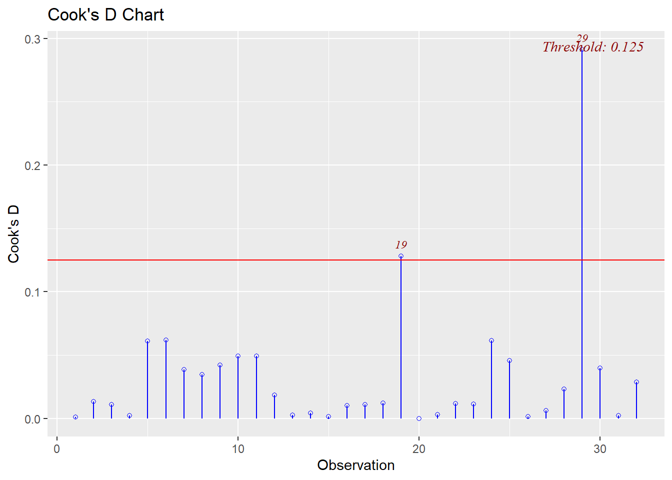

Above, we received a scatterplot. The vertical axis shows the calculated Cook’s distance for each observation and the horizontal axis shows each observation in order. The scatterplot also includes a horizontal red line which shows a threshold at which we might be concerned about an observation being an outlier. In the plot above, we see that observation 29 is clearly considered to be an outlier according to Cook’s distance. Observation 19 is also close to the threshold and might warrant further investigation later.

Cook’s distance tells us how influential each data point is in the calculation of the regression analysis. Our results tell us that observations 29 and 19 might be having more influence on our final results than most of the other observations in our data.

The threshold value is calculated as:

\(threshold = \frac{4}{\text{number of observations in dataset}} = \frac{4}{32} = 0.125\)

In R, we can calculate this with the following code:

4/nrow(d)

## [1] 0.125

The value above is 0.125. The red horizontal line in the scatterplot is also at 0.125. It is not necessary to manually calculate the threshold the way we just did above. It is sufficient to just look at the plot visually. Also—like most analogous situations in our study of statistics—note that this threshold value is not a hard and fast rule. You still might want to investigate other observations even if they are not about this threshold.

As an option, here is the code to calculate and save Cook’s distance for a regression model:

cooksd <- cooks.distance(reg1)

Above, we used the cooks.distance(...) function to calculate the Cook’s distances for all observations in our regression model reg1, but including reg1 as the argument in the function. We saved these calculated distances as cooksd.

You can see the saved Cook’s distance values by running the following command on your computer:

View(as.data.frame(cooksd))

Typically, you will not need to do anything beyond looking at the plot. However, there may be some situations in which it is useful to calculate the Cook’s distances and put them in a spreadsheet as demonstrated above, such as when you have a very large data set and you are not able to read the plot easily. For the purposes of our study of statistics in this textbook, looking at the plot visually is sufficient.

Now that we know that observations 29 and 19 might be suspicious, what do we do next? There is no single right answer, but a good first step is to run the regression model once again while excluding these observations. Then, we would compare the results of the two versions of the model to see if the results are different. If the results are not different, then we have additional support in favor of our one conclusion. If the results are different, we must make a decision about whether it is more appropriate to include or exclude the outliers in the regression model. This decision should be made by taking into account which version of our data best helps us answer our question of interest. When we report our results it is also important to transparently state the results of our outlier analysis and how we handled outliers in the end.

Of course, it is also important to use other methods of outlier identification before we make a final decision. Keep reading to see another way to identify outliers in a regression model.

6.3.2 DFFITs

Another measure of outliers and influence in a regression model is called DFFIT. Like Cook’s distance, this is also calculated for each observation in our dataset. We will not carefully examine this process. To summarize, the computer removes each observation one at a time, recalculates the regression, and sees how much the predicted values in the regression model change as a result of removing each observation. More specifically, DFFIT tells us how many standard deviations the predicted values change each time an observation is removed.¹³⁰

We can visualize the DFFITs for our regression model like this:

ols_plot_dffits(reg1)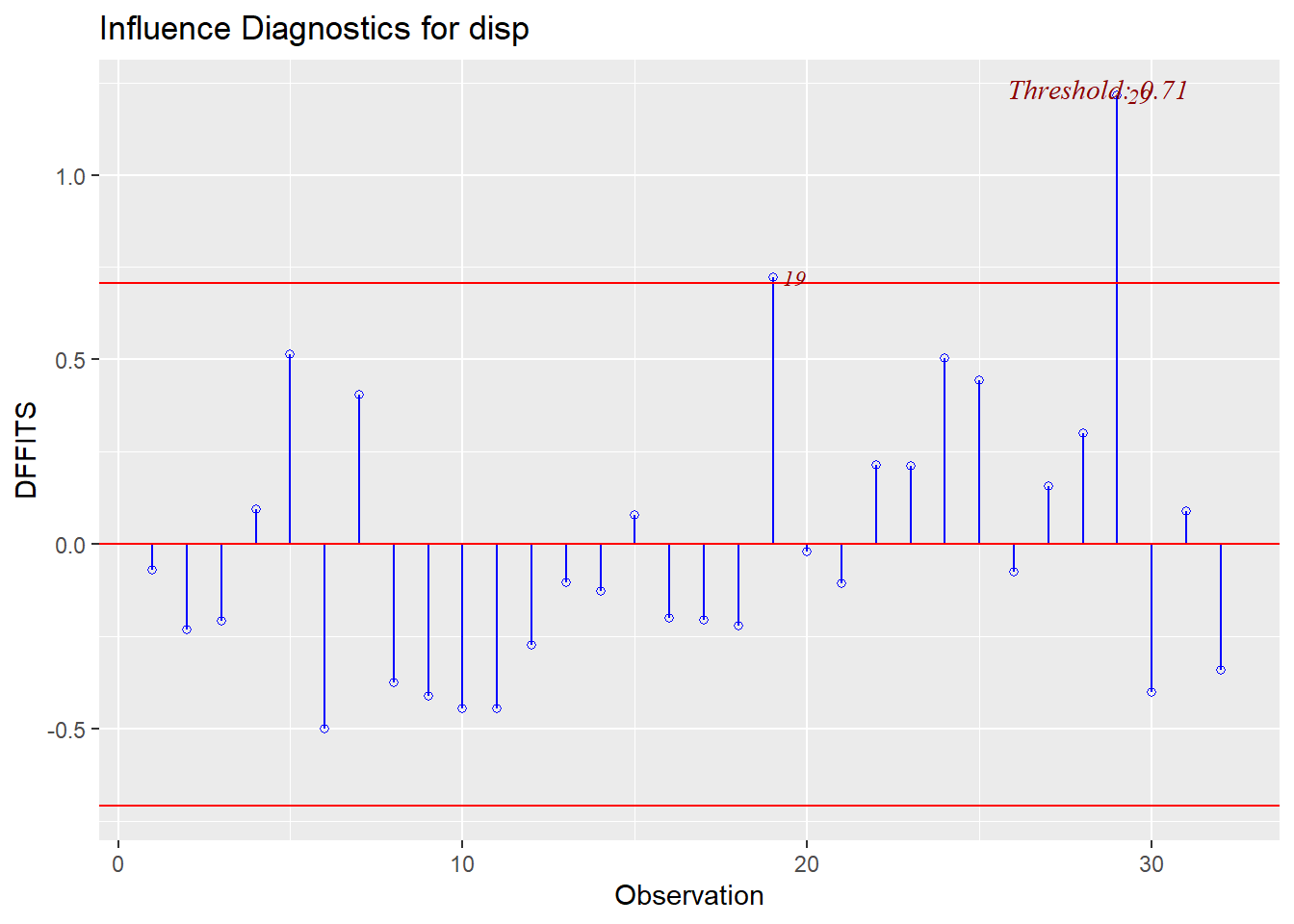

In the scatterplot above, we see DFFITs plotted against observation numbers, similar to our Cook’s distance plot. Red threshold lines are again drawn. The DFFITs method of detecting outliers also points to observations 29 and 19 as potentially problematic. These two points warrant further investigation and possible removal from our data.

If we want to calculate the DFFIT values and store them in R, we can use the following code:

dffits <- dffits(reg1)

And we could inspect them as a spreadsheet like this:

View(as.data.frame(dffits))

For our purposes, it will typically not be necessary to calculate these in R in a spreadsheet. Looking at the scatterplot should be good enough.

The threshold lines for DFFITs are calculated as:¹³¹

\(threshold = 2 * \sqrt{\frac{p}{n}} = 2 * \sqrt{\frac{4}{n}} = 0.71\)

• \(n =\) number of observations in our data. \(n=32\) in our example.
• \(p =\) number of independent variables in the regression model, counting the intercept as an independent variable. \(p=4\) in our example reg1.

0.71 is the same threshold we see in the scatterplot. Note that we consider outliers to be points greater than the threshold (0.71) or less than the negative of the threshold (-0.71). For example, if observation 6 had a slightly lower DFFIT value, it would be below the lower threshold line and would be considered an outlier.

We can calculate this in R with the following code:

p <- length(reg1$coefficients)
n <- nrow(d)
2*sqrt(p/n)

## [1] 0.7071068

Again, it is not necessary to manually calculate this threshold. You can usually just look at the lines on the plot for our purposes.

6.3.3 Studentized residuals plotted against leverage

Another useful way to examine potential outliers in our data with respect to a regression model is to plot the studentized residual against the leverage of each observation. Each of these metrics is summarized below:

• Studentized residual – This is a special type of residual error that is calculated for each observation in a regression model. This is calculated by removing each observation one at a time and calculating a regression equation on all of the other observations. A residual is then calculated for the removed observation by calculating a predicted value of that removed observation based on the regression equation that was created on all of the other observations (and then finding the difference between that predicted value and each observation’s actual value, as usual).¹³² This process is repeated for all observations and then these new residuals are standardized such that they can easily be compared to each other. An observation that has a studentized residual should be investigated.

• Leverage – Leverage is a number that is calculated for each observation based only on the independent variables. It is unrelated to the dependent variable. It is a measure of the extent to which each observation contains extreme values on one or more of the independent variables. An observation that has a high leverage value needs to be investigated in case it has undesirable influence on regression results.

It is common to plot studentized residuals against leverage, which we can do by using the ols_plot_resid_lev(...) function:

ols_plot_resid_lev(reg1)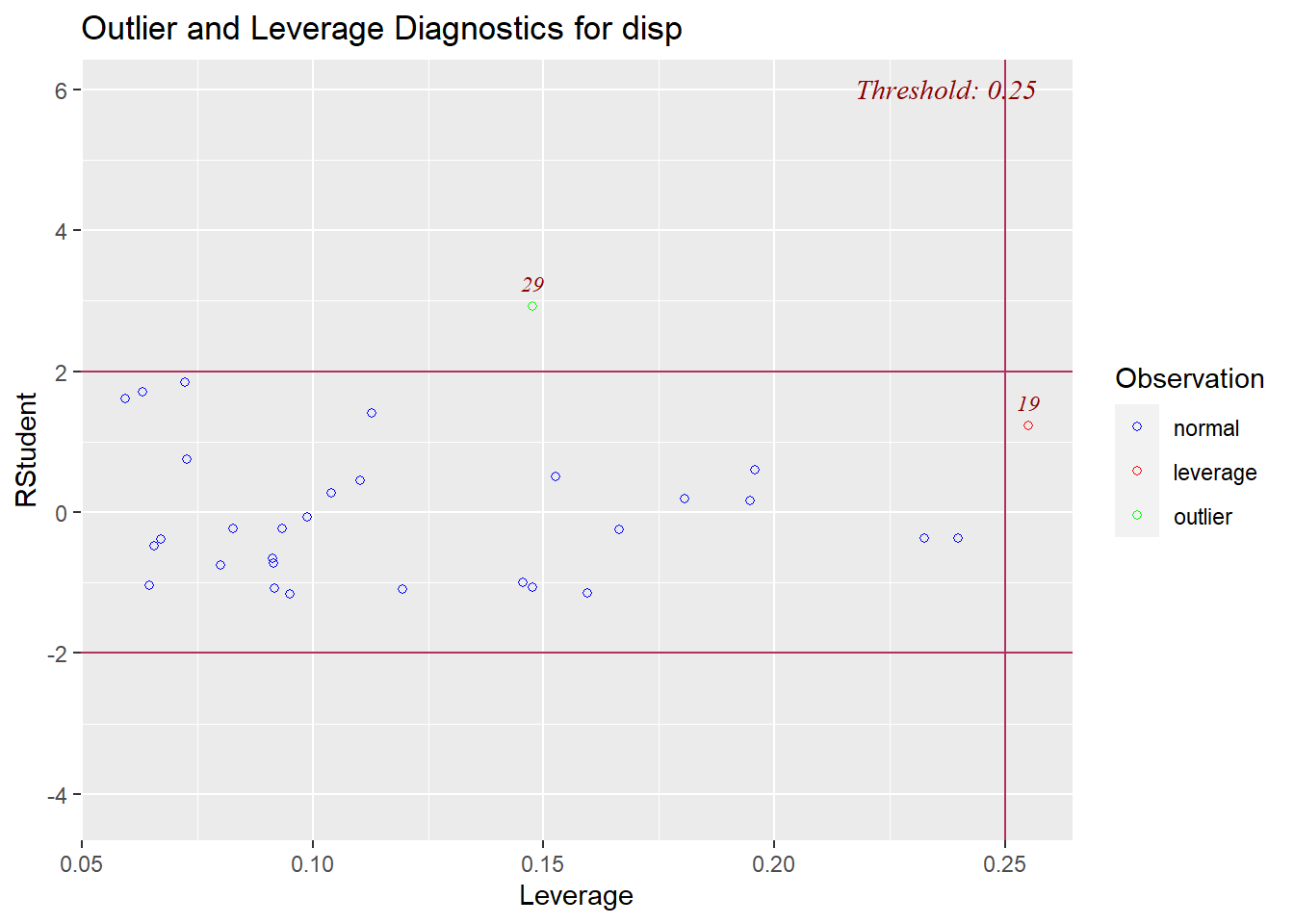

Above, the scatterplot we receive shows threshold lines for both studentized residuals and leverage. The observations that fall within all threshold lines are classified as normal, while those that fall outside of at least one threshold are marked as potentially problematic—either outlier or (high) leverage. As we have seen throughout this section, observations 29 and 19 are both marked as potentially problematic. They both need to be investigated to see if they warrant removal from our data.

We can calculate the studentized residuals with the following code:

d$resid.student <- rstudent(reg1)

Above, we added a variable called resid.student to our dataset d. resid.student contains the studentized residuals of our regression model for each observation. The rstudent(...) function calculates these for us when we provide our regression model reg1 as an argument.

Observations that have a studentized residual below -2 or above +2 are considered to be potentially problematic. These are where the red threshold lines are drawn on the plot we inspected earlier.

We can also calculate the leverage for each observation like this:

d$leverage <- hatvalues(reg1)

Above, we added a variable called leverage to our dataset d. leverage contains the leverage value of our regression model for each observation. The hatvalues(...) function calculates these for us when we provide our regression model reg1 as an argument.

The threshold for a problematic leverage value is sometimes considered to be two times the mean of all of the leverage values:¹³³

\(threshold = 2* \text{mean leverage} = 0.25\)

We can calculate this threshold for our regression model reg1 in R like this:

2*mean(d$leverage)

## [1] 0.25

As you can see, the horizontal red line on the scatterplot is drawn where the leverage is equal to 0.25.

Of course, you can inspect the calculated studentized residuals and leverage values with this code on your own computer:

View(d)

It is probably not necessary for you to know how to calculate the studentized residuals or leverage values. It is most important for you to be able to create the scatterplot above and understand how to interpret it.

6.3.4 DFBETAs

While most of the methods we use to identify potentially problematic observations focus on the regression model as a whole, is also possible to examine how individual observations may be influencing the estimation of specific estimates in our regression model. To do this, we calculate what are called DFBETA values for each independent variable for each observation. These values tell us separately for the independent variables and the intercept of our regression model if any observation might be having strong influence.

We can plot the DFBETAs for all observations using the ols_plot_dfbetas(...) with our regression model reg1 as the argument:

ols_plot_dfbetas(reg1)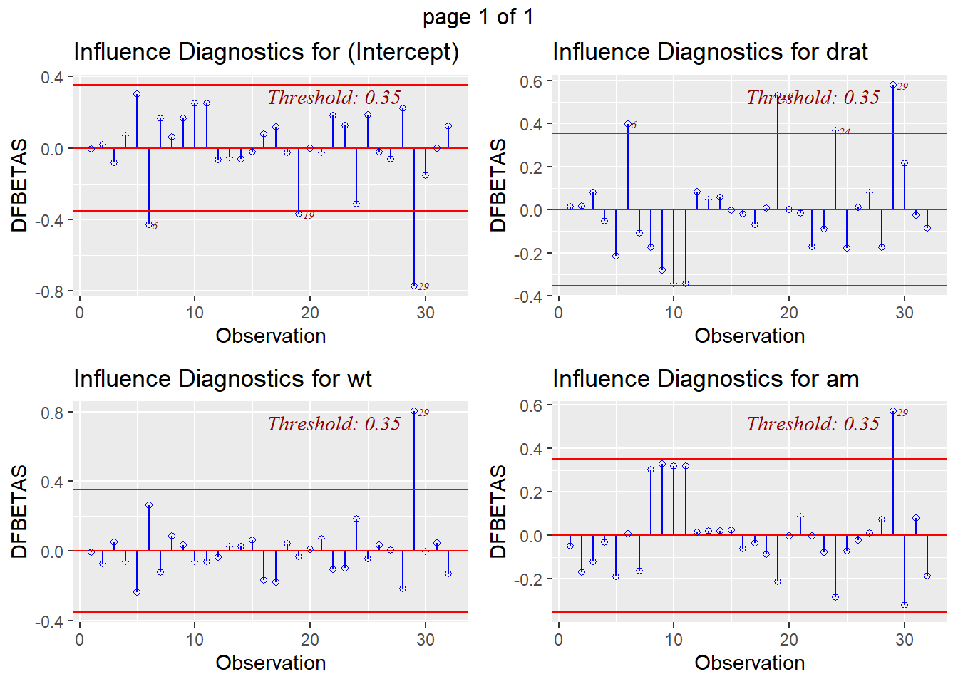

Above, we receive a scatterplot for each independent variable as well as the intercept. Observations that fall outside of the marked red thresholds warrant additional investigation.

Here is what we can gather from the plots above:

• Observations 6, 19, and 29 have high influence on the estimation of the intercept.
• Observations 6, 19, and 29 have high influence on the estimation of the relationship between disp and drat.
• Observation 29 has high influence on the estimation of the relationship between disp and wt.
• Observation 29 has high influence on the estimation of the relationship between disp and am.

A table of DFBETA values can be calculated with this code:

dfbeta.reg1 <- dfbetas(reg1)

Above, we created a new table¹³⁴ called dfbeta.reg1 which we created using the dfbetas(...) function which contained reg1 as its only argument.

This table can be viewed with the following code:

View(as.data.frame(dfbeta.reg1))

The threshold for potentially problematic DFBETA values for all estimated independent variables or intercepts is:

\(threshold = \frac{2}{\sqrt{\text{number of observations}}} = 0.35\)

We can calculate this in R with this code:

2/sqrt(32)

## [1] 0.3535534

We see that 0.35 is the same threshold used in the DFBETA scatterplots above. Any value below -0.35 or above +0.35 identifies a potentially problematic observation.

6.4 Specifying regression models

Earlier in this chapter, we learned a number of ways to modify regression models to better fit our data or answer a quantitative question. These included accounting for non-linear trends, modeling interactions, and identifying (and potentially removing) outliers. The process of deciding how to construct a regression model is called model specification. Model specification includes choosing which independent variables to include, deciding how to transform or interact those independent variables, and deciding if and how to modify your data before running the regression and interpreting the results. It is critical to specify a model that a) helps you answer your question correctly, b) is appropriate for the type of data and question you have, and c) will not cause you to reach a false or unsupported conclusion.

In this textbook, most of the time when we present a new analysis method, there is a single recommended way to analyze the data. As we continue our study of statistics and as you apply these methods on other questions and data, outside of this textbook, you will sometimes find ambiguity about what the best type of model is to fit your data and answer your question of interest. In general, if there are multiple reasonable ways for you to specify your regression model, I recommend that you run a number of different regression models to try to answer your question of interest. Then you should compare the results of these models to each other. If the results are the same, that provides extra support for the same conclusion. If the results are different, that is a clue that you need to dig deeper into what is going on, to figure out why the results are different even when you do your analysis in multiple reasonable ways.

If your results change depending on the regression model, this can also be due to what is called model dependence. This is a situation in which the specific analysis method you choose and the particular way in which you choose to specify your regression model might be causing you to find a particular conclusion, rather than that conclusion being the truth in your population of interest. As we continue to tackle more complicated questions and data in the rest of this textbook, we will also learn more about how to compare regression models to each other and how to avoid or minimize mistakes related to model specification or dependence.

Earlier in this chapter, we learned about transforming independent variables to model non-linear data and interacting independent variables to analyze relationships at the group level. We learned each of these methods in isolation. However, it is important to note that you can combine these methods together. For example, you could have a regression model in which some of the independent variables are squared (or transformed in some other way), others are interacted with each other, and others stand alone without being transformed or interacted. Theoretically, you can add an unlimited number of independent variables in various combinations of interactions¹³⁵ and transformations. This scenario is often not demonstrated when we are learning a new method, so it is important to keep in mind when you model data on your own in the future.

Earlier in this chapter, we looked at the following regression model called olsA which included an interaction between age and gender:

olsA <- lm(outcome ~ age + gender_male + gender_other + age.male  + age.other, data = d2)

Now let’s imagine that we have the following additional independent variables that we want to add to the regression model: years of education, years of education squared, race dummy variables, and weight in kilograms. Let’s say that we do not want to look at any interactions related to these additional independent variables.

Here is what this new regression model might look like:

olsA <- lm(outcome ~ age + gender_male + gender_other + age.male  + age.other + educyrs + educyrsSq + race_black + race_asian + race_other + weightkg, data = d2)

After running the model above, we would look at a regression result table the way we always do. We would see coefficient estimates for all of the independent variable terms above.

Here are some notes about how we would interpret the results:

• We would interpret the age and gender interaction term the way we did earlier in the chapter, just adding “controlling for all other independent variables.” For example: For every one year increase in age, outcome is predicted to increase by 0.96 units on average for females, controlling for all other independent variables.
• We would interpret the race dummy variables the same way that we would interpret dummy variables in any other situation, even though other independent variables are interacted or squared. For example: Black people are predicted to score ______ units higher than white people on average, controlling for all other independent variables. In this example, white people are the reference category.
• We would interpret the education and education squared variables the way we learned earlier in this chapter, just adding that we are now controlling for all other independent variables. For example: For people with years of education between 0 and 10 years, for every one year increase in education, outcome is predicted to increase on average, controlling for all other independent variables. This positive relationship between outcome and years of education gets less and less positive as we approach 10 years of education.

The decisions you make as you specify a regression model—including your choice of which independent variables to include and in which combinations—must be primarily driven by your question of interest. The whole reason we are learning to conduct quantitative analysis is to answer questions. So we cannot lose sight of this goal throughout the entire research process.

You have now reached the end of this chapter’s content and can proceed to the assignment that follows.

6.5 Assignment

In this assignment, you will practice modeling nonlinear data, modeling interaction terms, and detecting outliers or other potentially problematic observations in an OLS model.

6.5.1 Nonlinear Transformations

In this part of the assignment, you will practice using OLS linear regression to fit a non-linear trend in data. You will follow a similar procedure to the one presented earlier in this chapter to fit nonlinear data.

Please run the following code to load the dataset, called h:

if (!require(openintro)) install.packages('openintro')
library(openintro)

data(hsb2)
h <- hsb2

summary(h)

You can also run the command ?hsb2 to read more about the dataset, which is called the High School and Beyond survey.¹³⁶ You will use h as your dataset for this entire assignment.

For this section of the assignment, our question of interest is: What is the relationship between math score and writing score, controlling for socioeconomic status?

Please use the following variables:

• Dependent Variable: math
• Independent Variables: ses, write

Note that one of these independent variables is categorical and the other is numeric.

Task 1: Present a standardized dataset description for the dataset you are using for this assignment.

Task 2: Use the plot() command to make a scatterplot of the dependent variable plotted against the independent variable that is numeric.

Task 3: Use the boxplot() command to make a boxplot of the dependent variable plotted against the independent variable that is categorical.

Task 4: Run an OLS linear regression to see if these two independent variables are linearly associated or not with the dependent variable (do not yet try to fit a non-linear trend). Call this regression mod1.

Task 5: Generate residual plots for mod1. Interpret both the visual results and the numeric outputs.

Task 6: Add a squared term to the regression for the appropriate independent variable and run the regression. Call this mod2.

Task 7: Generate residual plots for mod2. Interpret both the visual results and the numeric outputs.

Task 8: Compare \(R^2\) values for mod1 and mod2.

Task 9: Based on the residual plots results alone, are both models—mod1 and mod2—trustworthy? Or only one or neither? You do not have to run diagnostic tests other than the residual plots.

Task 10: Write out the equation for mod2.

Task 11: Visualize the equation for mod2 into a graphing calculator to visualize it at https://www.desmos.com/calculator. Be sure to adjust the axes by clicking on the wrench in the top-right corner. Leave out the ses variable when you make this graph. You do not need to submit anything related to this task.

6.5.2 Interactions

Now we will turn to another research question, still based on our dataset h from above: Is the relationship between reading score and social studies score different for people with low, middle, and high levels of socioeconomic status, when controlling for science score and gender?

You will use an interaction term in an OLS model to answer this question. Note that reading score is the dependent variable. Also note that in this assignment, you should treat socioeconomic status as a categorical variable (the way it is in the original form of the data), not a continuous numeric variable. Then you will create dummy variables for each level of ses, the way we always do for categorical variables.

Task 12: Run an OLS regression model to answer the question of interest. Create a regression results table which includes 95% confidence intervals.

Task 13: Write out the full regression equation based on this output.

Task 14: Write the regression equation separately for each of the three ses groups. Present three equations.

Task 15: Use the interact_plot() function to visualize the results.

Task 16: Interpret each estimate—meaning all independent variables and the intercept—in the regression model for our sample. Be sure to clearly interpret and focus most on the interaction terms of socst and ses which help us answer our question of interest.

Task 17: Calculate the predicted value of reading score for each of the following people.

• Low socioeconomic status, female, 50 science score, 38 social studies score.
• Middle socioeconomic status, female, 50 science score, 38 social studies score.
• High socioeconomic status, female, 50 science score, 38 social studies score.

Task 18: Interpret each estimate in the regression model for our population of interest.

Task 19: What is the answer to our question of interest? Be sure to address our question for the population of interest primarily.

Task 20: The six figures below¹³⁷ show the population means for six experiments. For each one, indicate whether an A effect, a B effect, and/or an AxB interaction is present. Note that in some figures, more than one of these effects are present. This task is unrelated to all previous tasks. You will not use R for this task. Feel free to ask for help when doing this task.

6.5.3 Outliers

Earlier in this assignment, you created two regression models—one to model non-linear data and another to model an interaction. For this portion of the assignment, related to the identification of outliers in regression models, select ONE of the two regression models that you created earlier in the assignment and use that model for all of the tasks in this part of the assignment.

Task 21: Create a scatterplot to analyze Cook’s distance for your regression model. Briefly interpret the results.

Task 22: Create a scatterplot to analyze DFFITs for your regression model. Briefly interpret the results.

Task 23: Create a scatterplot to analyze studentized residuals and leverage for your regression model. Briefly interpret the results.

Task 24: Create a set of scatterplots to analyze DFBETAs for your regression model. Briefly interpret the results.

Task 25: Provide an overall conclusion to your analysis of outliers and potentially problematic observations in your regression model. Please also summarize what your next steps would be if this were an important project and you were required to create a trustworthy regression model with which you could report results. You do not actually need to do these steps, just briefly state what they would be.

6.5.4 Additional items

You have now reached the end of this week’s assignment. The tasks below will guide you through submission of the assignment, remind you of any other items you need to complete this week, and allow us to gather questions and/or feedback from you.

Task 26: You are required to complete 15 quiz question flashcards in the Adaptive Learner App by the end of this week.

Task 27: Please write any questions you have for the course instructors (optional).

Task 28: Please write any feedback you have about the instructional materials (optional).

Task 29: If you have not done so already, please email Anshul and Nicole with one or two times that might work well for you to do your Oral Exam #1. If you find yourself in an extenuating circumstance and would like to postpone your Oral Exam #1, please also email Anshul and Nicole about this.

Task 30: Knit (export) your RMarkdown file into a format of your choosing.

Task 31: Please submit your assignment to the D2L assignment drop-box corresponding to this chapter and week of the course. And remember that if you have trouble getting your RMarkdown file to knit, you can submit your RMarkdown file itself. You can also submit an additional file(s) if needed.

---

118. In fact, when \(R^2\) is so high with social science data, it can sometimes be a red flag that something is wrong. It may indicate that one of your independent variables is so similar to your dependent variable that it is not meaningful and/or useful to study the relationship between these two variables and the concepts that they measure.↩︎

119. This plot uses the function ggplot from the popular package ggplot2. You are not required to learn how to use ggplot in this class or how to make a plot like this.↩︎

120. In this case, gender is the only other independent variable. But there could have been more (that are not interacted).↩︎

121. In this case, age is the only other independent variable. But there could have been more (that are not interacted).↩︎

122. More experienced users of R may be aware of one or more shortcuts—which have not been mentioned so far in this textbook—that can be used to more efficiently include dummy variables in regression models. For now, I recommend against using such shortcuts, so that the process by which we convert a qualitative categorical variable into one or more numeric dummy variables can be fully understood and practiced.↩︎

123. The 0.96 estimate is the sum of the age and age.female estimates: \(0.22+0.74=0.96\)↩︎

124. A term is anything in between the plus or minus signs. In the equation \(a = 2b - rudolph + 43\), the \(2b\), \(rudolph\), and \(43\) are all terms on the right side of the equation.↩︎

125. This is an increase of -0.07 which is the same as a decrease of 0.07.↩︎

126. The 0.22 estimate is the sum of the age and age.male estimates: \(0.96-0.74=0.22\)↩︎

127. The 0.03 estimate is the sum of the age and age.nonbinary estimates: \(0.96-0.93=0.03\)↩︎

128. In this example, age is the only continuous numeric variable in our regression. In a more complicated regression model with multiple independent variables, we would have the option to choose which independent variable to put on the horizontal axis. Also note that we do not specify the dependent variable to put on the vertical axis of the scatterplot because the computer already knows what the dependent variable in the olsB model is.↩︎

129. Much of the code and interpretation from this section is adapted from: Measures of Influence. Accessed Feb 2021. https://cran.r-project.org/web/packages/olsrr/vignettes/influence_measures.html.↩︎

130. Measures of Influence. Accessed Feb 2021. https://cran.r-project.org/web/packages/olsrr/vignettes/influence_measures.html.↩︎

131. Zach. 13 Dec 2020. How to Calculate DFFITS in R. Accessed Feb 2021. https://www.statology.org/dffits-in-r/.↩︎

132. 9.4 - Studentized Residuals in Lesson 9: Influential Points in Stat 462, Applied Regression Analysis. Accessed Feb 2021. https://online.stat.psu.edu/stat462/node/247/.↩︎

133. Section “13.3.1 Leverage” in Applied Statistics with R. 30 Oct 2020. Accessed Feb 2021. https://daviddalpiaz.github.io/appliedstats/.↩︎

134. In this case, it is an R object called a matrix.↩︎

135. It is also possible to interact continuous variables with each other. It is not a rule that one variable has to be categorical (converted into dummy variables) and the other has to be continuous numeric. An example of this is not presented in this textbook, although this technique may occasionally be appropriate to help answer a question of interest.↩︎

136. The hsb2 data is part of the openintro package, which is why we loaded that package before using the data() command to load the data into R.↩︎

137. These figures came from Dr. Annie Fox at MGH Institute of Health Professions.↩︎