Chapter 3 Inference, Hypothesis Tests, and T-Tests

This week, our goals are to…

Review the process of inference, including the relationship between sample and population.
Review the basic logic of hypothesis testing.
Conduct a t-test on the type of data used in randomized controlled trials (RCTs).
Conduct all diagnostic tests of assumptions that are required for independent and paired⁴⁷ sample t-tests to determine if these results are trustworthy or not.

Announcements and reminders

Remember that you can use your own data for the assignments in this course. You are not forced to use the provided data. Feel free to discuss this with the instructors as necessary. You can also use your own data without asking first as long as you can accomplish all of the tasks with that data.

3.1 Inference, sample, and population

One of the most basic goals of quantitative analysis is to be able to use numbers to answer questions about a group of people. These questions often involve measuring a construct or examining a potential relationship.

Here are some examples of quantitative questions we might ask:

How many households in Karachi, Pakistan have a motorcycle?
Do physician assistant students in Massachusetts score higher on the Physician Assistant Clinical Knowledge Rating and Assessment Tool (PACKRAT) after their second year of training compared to after their first year of training?
In the United States of America, what is the relationship between the number of words a person knows and a person’s age?

To answer each of the questions above, we would need to first define and identify the following:

Question – What we are trying to answer using collected data, numbers, and quantitative analysis methods.
Population (also called population of interest) – The group about which we are trying to answer our question. This can be a group of people, objects, or anything else about which we can collect information.
Sample – A subgroup of the population of interest. Typically, it is not possible for us to collect data on all members of our entire population of interest, so we have to select a subgroup of the population of interest to analyze and collect data on. This subgroup is called our sample.
Inference – The process of analyzing the data in our sample to learn about our population. This process often involves making guesses or assumptions about the relationship between our sample and our population of interest. We want to be responsible practitioners of quantitative analysis when we conduct inference. Quite often, we will consider the assumptions we have made and we might realize that it would not be reasonable for us to make an inference to draw a conclusion about our population of interest using the sample that we have.
Inference procedure – A specific quantitative method that we will select which will allow us to make an inference, meaning use information about our sample to draw a conclusion about our population of interest. You will learn about many inference procedures during this course, including t-test, linear regression, and logistic regression. The inference procedure has to be selected carefully, such that it will allow us to answer our question and such that it is well-suited for the type of data we have. All limitations of our selected inference procedure need to be transparently communicated when we share our results. Frequently, we will try out multiple inference procedures to help us answer a single question. We will then compare the results from these multiple procedures and draw our conclusion carefully.⁴⁸ It is nice when multiple analytic approaches confirm the same result, but that doesn’t always happen.
Unit of observation – The level within your sample at which you collect your data. This is often the person or object. A unit of observation can also be thought of as an individual row in your data spreadsheet. What does each row of your dataset represent? The answer to this question is usually your unit of observation.

The concepts above may be confusing before you have some experience using them. Let’s start to build that experience using some examples. In the table below, we revisit the quantitative questions that were introduced earlier.

Selected concepts for each example quantitative research question:

Concept	Question 1	Question 2	Question 3
Question	How many households in Karachi, Pakistan have a motorcycle?	Do physician assistant students in Massachusetts score higher on the Physician Assistant Clinical Knowledge Rating and Assessment Tool (PACKRAT) after their second year of training compared to after their first year of training?	In the United States of America (USA), what is the relationship between the number of words a person knows and a person’s age?
Population	All households in Karachi.	All first and second year physician assistant students in Massachusetts.	All residents of the USA.
Sample	100 households in Karachi that we were able to survey.	First and second year physician assistant students at MGH Institute of Health Professions (MGHIHP)	28,867 residents of the USA surveyed and given a vocabulary test between 1978 and 2016.
Inference	Use data collected on motorcycle ownership in our sample (100 households in Karachi) to make guesses about motorcycle ownership in our entire population (all households in Karachi).	Use data in our sample (PACKRAT results of first and second year students at MGHIHP) to make a guess about our population of interest (PACKRAT performance of all physician assistant students in Massachusetts).	Determine the relationship between vocabulary test score and age in our sample (28,867 residents) and use this to guess about the nature of this relationship in our population of interest (all USA residents).
Inference procedure	Calculate percentage of households in our sample that have a motorcycle. Check if our sample is appropriately representative of our population; if so, assume that the percentage of households with motorcycles is the same in the population as in the sample. Calculate and report range of error on our estimate.	Compare PACKRAT performance of first year physician assistant students to that of second year students at MGHIHP, using a t-test. If the assumptions for a t-test result to be trustworthy for inference are met, t-test result can be reported as result for the entire population.	In sampled survey participants’ data, calculate the slope defining the relationship between vocabulary test score and age, using linear regression. If the assumptions for a linear regression result to be trustworthy for inference are met, linear regression result can be reported as result for the entire population.
Unit of observation	Household	Physician assistant student	Person

Most analytic methods presented in this textbook allow us to conduct the process of inference. In most cases, we will have a question of interest, a population in which we are interested in answering that question, and a sample of data that is drawn from that population. Most of the time, we will first answer our question of interest only within our sample. Then, we will do some diagnostic tests of assumptions. If our analysis passes all of these tests, then we can often use our results from our sample alone to answer our question of interest in our population. The process below illustrates this procedure.

Process of inferential quantitative analysis:

Ask a question
Identify population of interest
Gather data on a sample (subgroup) from the population
Answer question on sample using appropriate quantitative method
Run diagnostic tests of assumptions to see if results from sample can apply to entire population (and be used to infer the answer to the question for the population)
Report results about population, to the extent possible.

When we answer quantitative questions using the process described in this section, we often have to test hypotheses using hypothesis tests. Hypothesis tests allow us to weigh the quantitative evidence that is available to us and then responsibly draw a conclusion (or not) to our question of interest. Keep reading to learn about hypothesis tests!

3.2 Hypothesis tests

Hypothesis tests are one of the most basic tools we use in inferential statistics as we try to use quantitative methods to answer a question. They help us weigh the quantitative evidence that we have in favor or against a particular conclusion. More specifically, they tell us the extent to which we can be confident in a particular conclusion.

In this section, we will go through the basic logic and formulation of hypothesis tests and then introduce some more formal language and terms that we will be using frequently going forward.

3.2.1 Basic logic and formulation

Before we formalize how a hypothesis test works, we will look at a few examples to become familiar with the logic of hypothesis testing. Keep in mind that what you are about to read is a logic-based framework for problem-solving. It is not exclusively a process related to quantitative analysis.

For our first example, let’s pretend that there is a high jumper⁴⁹ named Weeda. We want to answer the following question: Can Weeda jump over a 7-foot bar?

One thing we could do is we could just guess and give an answer based on what we know about Weeda from before. However, as responsible quantitative researchers, we’re not going to do that. We’re going to be more strict. We are going to use the following analytic strategy: We will assume that Weeda can NOT jump over a 7-foot bar UNLESS we see convincing evidence that Weeda CAN do it.

This can be rewritten as a hypothesis test:

Null hypothesis – Weeda can not jump over a 7-foot bar. This is our default assumption if we don’t see any evidence to the contrary.
Alternate hypothesis – Weeda can jump over a 7-foot bar.

Next, we go to a sports facility to collect some data and we watch Weeda.

There are three possible outcomes:

Weeda tries to jump over the 7-foot bar and is able to do it. In this case, we reject the null hypothesis because we have evidence to support the alternate hypothesis.
Weeda tries to jump over the 7-foot bar and is not able to do it. In this case, we fail to reject the null hypothesis because we do not have evidence to support the alternate hypothesis.
Weeda never attempts to jump. In this case, we fail to reject the null hypothesis because we do not have evidence to support the alternate hypothesis.

So, what is the truth? Can Weeda jump over the 7-foot bar or not? Let’s unpack the situation:

Basically, if we have evidence that Weeda can jump over the 7-foot bar, then we conclude that the truth is that Weeda can jump over the 7-foot bar. And we reject the null hypothesis, which says that Weeda can’t accomplish the jump. We found convincing evidence against the null hypothesis.
If we do not have evidence that Weeda can jump over the 7-foot bar, then we don’t know the truth.⁵⁰ Maybe Weeda can do it but didn’t do it when we collected data. Or maybe Weeda can’t do it. We just don’t know. For this reason, when we do not have evidence to support the alternate hypothesis, we DO NOT say that we “accept” the null hypothesis. We NEVER EVER EVER “accept” the null hypothesis. Instead, we just fail to find evidence against the null hypothesis, leaving the truth unknown. So we say that we fail to reject the null hypothesis.

You might be wondering: What if our goal is to prove that Weeda cannot jump over the 7-foot bar? Well, we can’t do that. All we can do is say that we failed to find evidence that Weeda can jump over the 7-foot bar.

To review, here is what we did above:

Identify a question we want to answer.
Write null and alternate hypotheses.
Gather data/evidence.
Evaluate strength of evidence in favor of alternate hypothesis.
1. If evidence in favor of alternate hypothesis is strong enough, reject null hypothesis.
2. If evidence in favor of alternate hypothesis is not strong—or doesn’t exist at all—then we fail to reject the null hypothesis.

How strong does evidence have to be such that is strong enough to reject the null hypothesis? Now that we have covered the possible scenarios that can occur as we a) use evidence to b) conduct a hypothesis test to c) answer a question, we can start to consider how this process relates to quantitative questions specifically and how we will use numbers to evaluate the extent or strength of our evidence in favor of the alternate hypothesis. This will be addressed in the next section!

In the example above, we used a framework for hypothesis testing but we did not mention inference. Below, we will discuss how we can use the hypothesis test framework for the purposes of inference (using a sample of data to make a guess about a population).

3.2.2 Formal language and terms

In the previous section, you read an example of the use of evidence and a hypothesis test to answer a question. Now, we will build on that framework and consider how it can help us specifically with quantitative analysis. To do this, we will use another example.

Imagine that we want to determine if a medication tablet is effective in lowering patients’ blood pressure over the course of 30 days. So, we enroll 100 patients as subjects into a study. 50 are in the treatment group and receive the medication. The other 50 are in the control group and do not receive the medication. At the end of the 30-day experiment, we see if the blood pressure of the 50 subjects in the treatment group decreased more than the blood pressure of the 50 subjects in the control group.

The diagram below summarizes this quantitative research design:

Let’s specify some now-familiar characteristics of this research design:

Question: Does the blood pressure medication reduce our patients’ blood pressure?
Population of interest: All patients with high blood pressure.
Sample: 100 patients with high blood pressure.
Data/evidence: Collected during randomized controlled trial.
Dependent variable: change in blood pressure over 30 days.
Independent variable: experimental group (meaning membership in treatment or control group).
Unit of observation: Patient
Hypotheses
- Null hypothesis: The blood pressure medication does not work, meaning that there will be no difference between the improvement in the treatment and control groups on Day 30.
- Alternate hypothesis: The blood pressure medication does work, meaning that there will be a significant difference between the improvement in the treatment and control groups on Day 30.

Now we will re-write the hypotheses above in a slightly more technical way:

Null hypothesis ($H_0$): The change in blood pressure in the treatment group will be equal to the change in blood pressure in the control group, in our population of interest.
Alternate hypothesis ($H_A$): The change in blood pressure in the treatment group will not be equal to the change in blood pressure in the control group, in our population of interest.

Basically, the null hypothesis is saying that the two groups—treatment and control—have the same outcome. The alternate hypothesis is saying that these two groups have different outcomes. Note that $H_0$ is a common way to write null hypothesis and $H_A$ is a common way to write alternate hypothesis.

To conduct a hypothesis test like the one we have set up above, we will usually choose a particular inference procedure to run in R and then we will receive results which might include an effect size, confidence interval for the effect size, and a p-value. We can answer our question of interest and reach a conclusion for our hypothesis test by interpreting these results.

Below, we will define effect size, confidence interval, and p-value. It is natural for these concepts to feel unclear even after reading the descriptions below. You will gradually start to understand them better as you encounter more examples and run analyses of your own.

Please note that we will now be using the hypothesis testing framework for the purposes of inference. For the rest of our study of quantitative analysis, hypothesis tests will always be used as part of an inference procedure in which we attempt to use a sample of data to make guesses (inferences) about a population. As you will read below, confidence intervals always tell us the range of possibilities of a particular estimate in our population of interest. Likewise, p-values tell us a probability related to our hypothesis test for our population of interest.

3.2.2.1 Effect size

Effect size means how large or small an outcome of interest is. In the context of our blood pressure medication example, if systolic blood pressure in the treatment group goes down by 10 mmHg on average, while systolic blood pressure in the control group goes down by 1 mmHg on average, the effect size of the medication in our sample of 100 subjects is $10-1=9 \text{ mmHg}$. It is then up to the researcher to decide if an effect size of 9 mmHg within the 100 sampled subjects is a meaningful effect size or not.

Imagine if the treatment group’s systolic blood pressure decreased by 1.5 mmHg while the control group’s systolic blood pressure decreased by 1 mmHg. Then the effect size of the medication in our sample of 100 subjects is $1.5-1=0.5 \text{ mmHg}$. Such a small effect size is probably not clinically meaningful, although it would still be up to the researcher to decide.

In both of the scenarios above—effect sizes of 9 or 0.5 mmHg—if we had strong enough evidence, we would reject the null hypothesis, because the treatment and control group results were not equal. This means that even if we do reject the null hypothesis, it still doesn’t necessarily mean that we got a meaningful result. A quantitative researcher has to also consider the size of the difference—in this case between treatment and control groups—that caused us to reject the null hypothesis and whether that size means anything or not.

In most quantitative analyses, we are not only interested in the effect size in an outcome of interest within our sample. Rather, we want to use data about our sample to determine the effect size in our outcome of interest in the entire population from which our sample was drawn (selected). In the context of our example, this means that we not only want to see if the medication is associated with a decrease in blood pressure in our sample of 100 subjects. Rather, we want to use our results from our sample of 100 subjects to determine if the medication is associated with a decrease in blood pressure in the entire population of patients who have high blood pressure.

While we are able to use subtraction to calculate an exact average effect size—either 9 or 0.5 mmHg in our scenarios above—for just our sample of 100 subjects, we cannot calculate an exact effect size for the entire population of patients with high blood pressure. Instead, all we can do is use statistical theory—which we are relying on the computer to implement for us—to generate a range of possible effect sizes in the entire population. We refer to this range of possibilities as a confidence interval.

3.2.2.2 Confidence interval

A confidence interval is a range of numbers that tells us plausible values of an outcome of interest in the population that we are trying to infer about. In our blood pressure example, perhaps we would find that while the effect size (of taking the medication) in our sample of 100 subjects is 9 mmHg, we are 95% certain that the effect size (of taking the medication) in the entire population is between 2 and 16 mmHg. This is called the 95% confidence interval. This means that we are 95% certain that the true effect of the medication on systolic blood pressure in the entire population of interest would have been no lower than 2 mmHg and no higher than 16 mmHg.

Now imagine that we were less certain about the association between taking the medication and blood pressure reduction. Imagine that the 95% confidence interval had been from -2 to 20 mmHg. In this case, the direction of the association is also in question. When the 95% confidence interval crosses 0, it means that we don’t even know the direction of the effect size in the population. If we gave this medication to the entire population, it is possible that their blood pressure would get better and also possible that it would get worse.

Confidence intervals are directly related to p-values, which are discussed below.

3.2.2.3 p-value

A p-value—sometimes just called p—is a number that is reported as a result of a hypothesis test. More specifically, the p-value is a probability that can be between 0 and 1. The p-value addresses a given hypothesis test for our population of interest, never for our sample of data.⁵¹

All p-values are the result of a hypothesis test in which we have a null hypothesis and are trying to determine if we have strong enough evidence to reject that null hypothesis in favor of an alternate hypothesis. The p-value tells us how strong or weak this evidence is.

1-p =

our level of confidence in the alternate hypothesis being true.
the probability that the alternate hypothesis is true
the strength on a scale from 0 to 1 of evidence in favor of the alternate hypothesis.

p =

the probability that rejecting the null hypothesis was a mistake (or would be a mistake if we did it).
the probability of committing a Type I error (see below).
the probability that the scenario in the alternate hypothesis occurred due to random chance, rather than the alternate hypothesis being the truth.⁵²

Here are some examples:

If $p=.03$ and $1-p=0.97$, this means that we are 97% confident in the alternate hypothesis. And there is a 3% chance that if we reject the null hypothesis, doing so (rejecting the null hypothesis) was a mistake. There is a 3% chance of Type I error (see below).
If $p=.43$ and $1-p=.57$, this means that we are 57% confident in the alternate hypothesis. And there is a 43% chance that if we reject the null hypothesis, doing so (rejecting the null hypothesis) was a mistake. There is a 43% chance of Type I error (see below).

And here are some guidelines to keep in mind about p-values:

The threshold for your p-value at which we will reject the null hypothesis is called an $\alpha\text{-level}$, pronounced “alpha level.” If $p < \alpha$—meaning if the p-value is below the alpha level—we reject the null hypothesis.
An alpha level is the threshold for what is commonly called statistical significance. This term can be misleading and we should try to avoid using it without providing additional context. If results of a hypothesis test are “statistically significant,” it does not necessarily mean that they are meaningful in a tangible or “real world” sense. Effect sizes, confidence intervals, and p-values all need to be considered together before answering a quantitative question. Diagnostic metrics and tests that are specific to each inference procedure also need to be taken into consideration before a conclusion can be drawn.
A commonly used alpha level is 0.05. In this common scenario, the null hypothesis is rejected when $p \le 0.05$. This is equal to 95% certainty (or more) and 5% probability (or less) of rejecting the null hypothesis being a mistake.
Higher p-values mean more uncertainty, meaning lower confidence in the alternate hypothesis. Higher p-values correspond to larger—and often inconclusive—confidence intervals.
Lower p-values mean more certainty, meaning higher confidence in the alternate hypothesis. Lower p-values correspond to smaller—and more definitive—confidence intervals.

3.2.3 Type I and type II errors in hypothesis testing

When we formulate a hypothesis test and reach a conclusion to that test, there are two types of errors we can make. These can be referred to as Type I and Type II errors, summarized below. I personally find these terms difficult to remember and not as useful as simply thinking through the concepts myself. It is optional (not required) for you to memorize these terms for the two types of error.

Possible errors in hypothesis testing:

Type I error: Reject the null hypothesis when it is really true.
Type II error: Fail to reject the null hypothesis when it is really false.

Remember: The p-value is the calculated probability that we made a mistake by rejecting the null hypothesis. In more technical terms, the p-value is the probability that we are making a Type I error. But you don’t need to think about it that way or memorize this. The key is to just remember that the p-value is the probability that if we reject the null hypothesis, doing so (rejecting the null hypothesis) is a mistake.

Now that we have examined how to formulate and conduct hypothesis tests at a conceptual level, let’s learn how to run one type of hypothesis test—a t-test—in R and interpret its results!

3.3 T-tests

A t-test is one of the most basic ways to determine if there is a difference between two groups in an outcome of interest. T-tests can be used to compare independent samples of data, where the observations in each comparison group are separate; and they can also be used for paired data, where the goal is to determine if there is a difference in an outcome of interest measured twice on the same observations. In this part of the chapter, we will learn how to conduct both types of t-tests and also examine the conditions under which we can or cannot trust our t-test results.

3.3.1 Independent samples t-test

An independent samples t-test is used when you have an outcome from two separate groups that you want to compare. More specifically, a t-test compares means from two different groups. The blood pressure medication example from earlier in this chapter is again applicable here. We want to compare two separate groups—treatment and control—to see if their mean change in blood pressure over 30 days is the same or different.⁵³

Let’s examine this data ourselves in R. We can run the following code to load the data:

treatment <- c(-8, -14.8, -6.8, -11.6, -10.2, -11.6, -4.8, -6.5, -9.9, -17.2, -10.7, -11.9, -8.7, -11.6, -8.6, -8.3, -10.9, -14.1, -8.8, -12.4, -14.1, -16.8, -1.8, -10.8, -15.1, -8.5, -11.2, -9.8, -10.9, -12.8, -9.2, -10.1, -12.2, -8.8, -8.5, -7.5, -10.2, -6.2, -11.4, -8.1, -15.3, -6.3, -7.2, -5.9, -13.4, -16.8, -10.7, -10.9, -12.9, -13.1)

control <- c(0, -3.5, -2.6, 3.7, -1.1, -0.6, -0.3, -1.5, 4.9, -1.8, -0.3, 0.2, -0.6, -6, -4.1, -0.5, -2.6, 0.4, 0.5, 1.9, -1, -0.1, 1.6, -3.2, -1, -3.7, 1.8, -4.2, 1, -2.2, 2, 5.5, 1.5, 1, 3.7, -1.5, -3.3, -2.7, -4.3, -7, -1.4, 5.2, 3.8, 4.6, -1.5, 2.1, -5.1, 0.5, 3.5, -0.7)

bpdata <- data.frame(group = rep(c("T", "C"), each = 50), SysBPChange = c(treatment,control))

Here is what we asked the computer to do for us above:

treatment <- c(...) – Create a column⁵⁴ of data (that is not part of any dataset⁵⁵) called treatment which contains 50 numbers. The 50 numbers are given by us to the computer inside of the c(...) portion of the command. The c is how a new column of data is defined in R.
control <- c(...) – Create a column of data (that is not part of any dataset) called control which contains 50 numbers, again defined using the c(...) notation.
bpdata <- data.frame(...) – Create a new dataset (technically called a data frame in R) with two variables (columns): group and SysBPChange (which stands for systolic blood pressure change).
- group = rep(c("T", "C"), each = 50) – Create a variable in the new dataset called group which will have 100 observations (rows). Observations in the first 50 rows will have a value of T and observations in the next 50 rows will have a value of C.
- SysBPChange = c(treatment,control)) – Create a variable in the new dataset called SysBPChange which will contain the values in the already-existing column of data called treatment and then the values in the already-existing column of data called control.

It is not essential for you to fully understand the commands above or use them in the future without explicit guidance.

Now bpdata, treatment, and control should appear in your Environment tab in RStudio. You can run the following commands to inspect these three new items:

View(bpdata)
View(treatment)
View(control)

Remember: Do not leave the View(...) commands above in your RMarkdown file, because doing so may cause problems when you try to Knit (export) your work!

Using the code below that we have used before, we can examine the dataset that we just created:

if (!require(dplyr)) install.packages('dplyr')
library(dplyr)

dplyr::group_by(bpdata, group) %>% 
dplyr::summarise(
  count = n(), 
  Mean_SysBPChange = mean(SysBPChange, na.rm = TRUE),
  SD_SysBPChange = sd(SysBPChange, na.rm = TRUE)
  )

## # A tibble: 2 × 4
##   group count Mean_SysBPChange SD_SysBPChange
##   <chr> <int>            <dbl>          <dbl>
## 1 C        50            -0.38           2.95
## 2 T        50           -10.5            3.22

Above, we can see that we have successfully created the dataset bpdata in which there are 50 observations in the treatment group—identified as T—and their mean change in systolic blood pressure was -10.5 mmHg, with a standard deviation of 3.2 mmHg. And there are 50 observations in the control group—identified as C—and their mean change in systolic blood pressure was -0.4 mmHg, with a standard deviation of 2.9 mmHg.

We can also visualize our data in bpdata using a boxplot:

boxplot(SysBPChange~group,bpdata)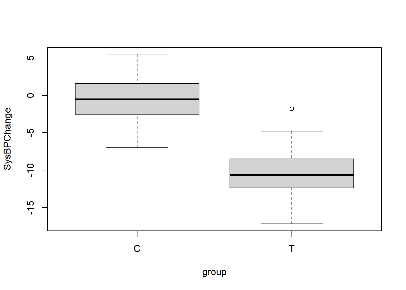

Note that we could also create the very same boxplot that you see above by running the following code:

boxplot(control,treatment)

In the code above, we give the computer the two columns of data separately for treatment and control groups, instead of giving the computer our data within a single dataset. You can try running this on your computer if you would like.

We are now ready to run an independent samples t-test.

The null hypothesis for this t-test is that the means of SysBPChange are equal in the treatment and control groups. We can write the null hypothesis like this:

\[H_0\text{: } \mu_T = \mu_C\]

In the notation above, $\mu$ represents the population mean (not sample mean) of our outcome of interest. $\mu_T$ is the population mean (not sample mean) of SysBPChange in our treatment group and $\mu_C$ is the population mean (not sample mean) of SysBPChange in our control group.

Another way to write this very same null hypothesis is like this:

\[H_0\text{: } \mu_T - \mu_C = 0\]

The alternate hypothesis is as follows:

\[H_A\text{: } \mu_T \ne \mu_C\]

\[H_A\text{: } \mu_T - \mu_C \ne 0\]

Note that for this independent samples t-test, our hypotheses relate to the population means of our treatment and control groups, not our sample means. It is important to solidify this concept before we continue. There are two populations that we are interested in learning about:

Those patients who receive the blood pressure medication. We have a sample of only 50 such patients and we know that their systolic blood pressure dropped by 10.5 mmHg on average. 10.5 is the sample mean. We do not know what happened to the blood pressure of the entire population of people who took the medication. The population mean is unknown.
Those patients who do not receive the blood pressure medication. We have a sample of only 50 such patients and we know that their systolic blood pressure dropped by 0.4 mmHg on average. 0.4 is the sample mean. We do not know what happened to the blood pressure of the entire population of people who did not take the medication. The population mean is unknown.

We already know that there is a difference of $10.5-0.4=10.1 \text{ mmHg}$ in our sample means. That is not what we are trying to learn from our t-test. Instead, we are trying to learn about the difference in the population means of these two types of people (those who received the medication and those who didn’t in the entire populations from which our 50-patient samples were selected).

We want to answer the question: If we were to hypothetically do an enormous experiment in which ALL patients with high blood pressure were subjects, how much of a difference (if at all) would we see in systolic blood pressure change between those who did and didn’t receive the medication?

We are trying to answer this question using our tiny study of 50 treatment subjects, 50 control subjects, and a t-test.

Now that we have clarified what exactly we are doing, let’s review the hypotheses in plain words. We start with the assumption—null hypothesis—that there is no difference in systolic blood pressure change between those who did and did not receive the medication in the entire population. If we find evidence that there is a difference, we will reject the null hypothesis in favor of the alternate hypothesis, which states that there is a difference in systolic blood pressure change between those who did and did not receive the medication in the population. If we do not find any evidence that the systolic blood pressures of those who did and did not take the medication in the population are different, we fail to reject the null hypothesis.

Now it is time to run our t-test in R, using the code below:

t.test(SysBPChange ~ group, data = bpdata)

## 
##  Welch Two Sample t-test
## 
## data:  SysBPChange by group
## t = 16.354, df = 97.233, p-value < 2.2e-16
## alternative hypothesis: true difference in means between group C and group T is not equal to 0
## 95 percent confidence interval:
##   8.872546 11.323454
## sample estimates:
## mean in group C mean in group T 
##          -0.380         -10.478

Here’s what we asked the computer to do with the code above:

t.test(...) – Run an independent samples t-test.
SysBPChange ~ group – Our outcome variable of interest—which we could also call our dependent variable—is SysBPChange. Our group identification variable—which also could be called our independent variable—is group.
data = bpdata – The dataset containing the variables used for this t-test is called bpdata.

Note that we could also run the following code to conduct the very same t-test (the results are not shown):⁵⁶

t.test(control,treatment)

And now we can interpret the results of the t-test from the output we received, pending the diagnostic tests later in this section:

The 95% confidence interval of the effect size in the population is 8.9–11.3 mmHg. This means that there is a 95% chance that in the entire population (not our sample of 100 subjects), people who take the medication improve (decrease) their systolic blood pressure by at least 8.9 mmHg and at most 11.3 mmHg on average, relative to those who don’t take the medication.
The p-value is extremely small, lower than 0.001.⁵⁷
We have sufficient evidence—pending the diagnostic tests later in this section—to reject the null hypothesis and conclude that in the population, the systolic blood pressures of those who take the medication reduce more than the systolic blood pressures of those who do not take the medication, on average.

Before we can consider the results of the t-test above to be trustworthy, we must first make sure that our data passes a few diagnostic tests of assumptions that must be met. These assumptions are discussed later in this section.

3.3.1.1 Example with uncertain confidence interval and high p-value

Below, the t-test procedure from above is repeated with an example in which we fail to reject the null hypothesis. All details are the same except for the outcome data for the treatment group, which have been modified for illustrative purposes.⁵⁸

You can copy and run the code below to follow this example.

treatment <- c(-8, -14.8, -6.8, -11.6, -10.2, -11.6, -4.8, -6.5, -9.9, -17.2, -10.7, -11.9, -8.7, -11.6, -8.6, -8.3, -10.9, -14.1, -8.8, -12.4, -14.1, -16.8, -1.8, -10.8, -15.1, -8.5, -11.2, -9.8, -10.9, -12.8, -9.2, -10.1, -12.2, -8.8, -8.5, -7.5, -10.2, -6.2, -11.4, -8.1, -15.3, -6.3, -7.2, -5.9, -13.4, -16.8, -10.7, -10.9, -12.9, -13.1)+9.5

control <- c(0, -3.5, -2.6, 3.7, -1.1, -0.6, -0.3, -1.5, 4.9, -1.8, -0.3, 0.2, -0.6, -6, -4.1, -0.5, -2.6, 0.4, 0.5, 1.9, -1, -0.1, 1.6, -3.2, -1, -3.7, 1.8, -4.2, 1, -2.2, 2, 5.5, 1.5, 1, 3.7, -1.5, -3.3, -2.7, -4.3, -7, -1.4, 5.2, 3.8, 4.6, -1.5, 2.1, -5.1, 0.5, 3.5, -0.7)

bpdata <- data.frame(group = rep(c("T", "C"), each = 50), SysBPChange = c(treatment,control))

The following boxplot helps us quickly understand this new data:

boxplot(SysBPChange ~ group, data = bpdata)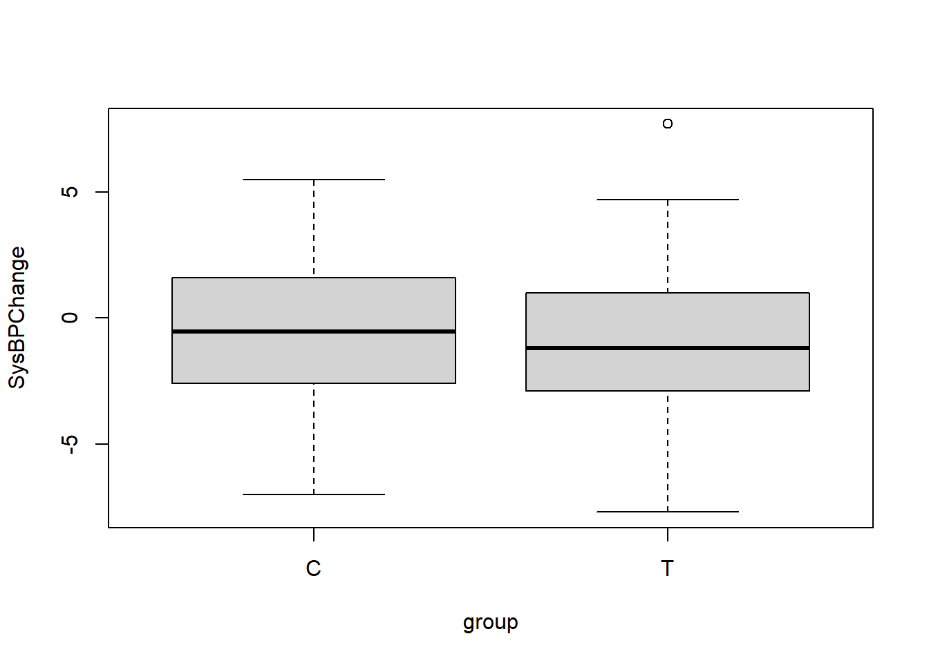

In this new version of the data, the medication did not make a difference in the treatment group, as the boxplot above shows.

Our hypotheses are the same as before:

$H_0\text{: } \mu_T = \mu_C$
$H_A\text{: } \mu_T \ne \mu_C$

And now we again run the t-test:

t.test(SysBPChange ~ group, data = bpdata)

## 
##  Welch Two Sample t-test
## 
## data:  SysBPChange by group
## t = 0.96848, df = 97.233, p-value = 0.3352
## alternative hypothesis: true difference in means between group C and group T is not equal to 0
## 95 percent confidence interval:
##  -0.6274544  1.8234544
## sample estimates:
## mean in group C mean in group T 
##          -0.380          -0.978

We can interpret the results of the t-test from the output we received, pending the diagnostic tests later in this section:

The 95% confidence interval of the effect size in the population is -0.6–1.8 mmHg. This means that there is a 95% chance that in the entire population (not our sample of 100 subjects), people who take the medication worsen their systolic blood pressure by at most 0.6 mmHg and improve it by at most 1.8 mmHg on average, relative to those who don’t take the medication. In this situation, the 95% confidence interval includes the number 0, meaning that we do not know if this is a negative (meaning that the medication makes the blood pressure of patients who take it worse than the blood pressure of patients who do not), zero (meaning that those who do and do not take the medication have the same blood pressure outcomes), or positive (meaning that the medication makes the blood pressure of patients who take it better than the blood pressure of patients who do not) trend. This is an inconclusive result.
The p-value is 0.34, which is quite large. This means that we have very low confidence in the alternate hypothesis.
We do not have sufficient evidence to reject the null hypothesis and conclude that in the population, the systolic blood pressures of those who take the medication reduce more than the systolic blood pressures of those who do not take the medication, on average.
We fail to reject the null hypothesis.

Note once again that before we can consider the results of the t-test above to be trustworthy, we must first make sure that our data passes a few diagnostic tests of assumptions that must be met. These assumptions are discussed later in this section.

3.3.2 Paired sample t-test

A paired sample t-test compares an outcome of interest that is measured twice on the same set of observations. Another name for a paired sample t-test is a dependent sample t-test (as a counterpart to the independent samples t-test we learned earlier). More specifically, the paired sample t-test compares the means of an outcome of interest that is measured twice within a single sample.

We will use an example to practice using a paired samples t-test. Imagine a situation in which 50 students are sampled from a larger population of students. These students are learning a particular skill. They are first pre-tested on their initial ability to perform the skill, then they participate in an educational intervention to improve their abilities to do the skill, and finally they take a post-test at the end of the procedure. We want to know if students in the larger population of students are able to perform the skill better after they participate in the educational intervention than before.⁵⁹ Since the two means—pre-test and post-test scores—we want to compare come from the same observations (students), a paired sample t-test is the correct inference procedure to use.

The research design is diagrammed in the chart below:

Now that we have identified a question to answer, let’s load our data into R using the following code.

post <- c(82.7, 71.7, 66.9, 67.9, 87.3, 65.5, 72.2, 81.2, 65.2, 79.1, 80.9, 94.6, 83.7, 76.8, 78.5, 70.4, 61.4, 93.3, 70.8, 71.7, 77.4, 70.8, 65.7, 69.6, 72.4, 73.3, 81.8, 71.6, 73.6, 72.8, 84.5, 73.3, 67.1, 80.7, 82.5, 84.1, 86.1, 84.7, 73.8, 74.5, 70.7, 80.5, 80.6, 61.2, 81.1, 78.6, 67.3, 67.6, 77.2, 66.8)

pre <- c(55.4, 82.8, 88.1, 74.4, 64.9, 73.9, 90.6, 90.6, 86.8, 83.5, 85.4, 87.3, 69.1, 84.4, 69.4, 38.5, 64, 67.5, 68, 86.8, 81.5, 56.6, 51.9, 65.5, 82.4, 65.3, 81.8, 58.9, 60.9, 66.1, 72.7, 45.5, 69.6, 70.1, 79.7, 68.4, 75.7, 39.3, 75, 63.9, 76.7, 67.2, 71.6, 62.9, 76.5, 90.1, 66.8, 71.8, 77, 65.2)

tests <- data.frame(pre,post)

Above, we created a dataset called tests which contains 50 observations (students, in this case). The dataset tests contains the variable pre, which holds all of the pre-test scores; and tests contains the variable post, which holds all of the post-test scores.

We can use familiar commands to describe our data:

summary(tests$pre)

##    Min. 1st Qu.  Median    Mean 3rd Qu.    Max. 
##   38.50   65.22   70.85   71.36   81.72   90.60

sd(tests$pre)

## [1] 12.47582

summary(tests$post)

##    Min. 1st Qu.  Median    Mean 3rd Qu.    Max. 
##   61.20   70.47   73.70   75.47   81.05   94.60

sd(tests$post)

## [1] 7.721632

We can visualize the pre and post-test scores using a boxplot:

boxplot(tests$pre,tests$post)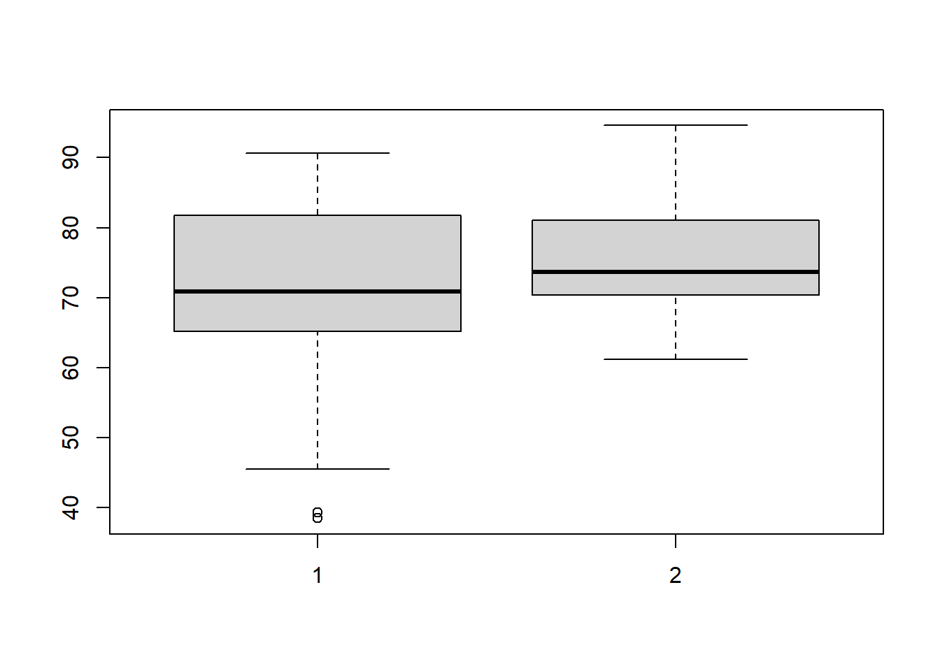

We can now write hypotheses for the paired sample t-test that we will use:

$H_0\text{: } \mu_{pre} = \mu_{post}$. The null hypothesis is that in the population of students from which the sample of 50 students were selected, students’ pre-test and post-test scores are the same on average.
$H_A\text{: } \mu_{pre} \ne \mu_{post}$. The alternate hypothesis is that in the population of students from which the sample of 50 students were selected, students’ pre-test and post-test scores are not the same on average.

As with the independent samples t-test, our hypotheses relate to the population from which our sample was selected, rather than our sample itself. Our goal is to find out if the educational intervention is associated with an improvement in test score in the entire population of students, not only in our sample of 50 students. We already know that in our sample of 50 students, the average pre-test score is 71.4 test points and the average post-test score is 75.5 test points; so the average difference is 4.1 test points. But what is this difference in our population? That’s what the paired sample t-test will help us figure out, below.

We can run the following code to run our paired sample t-test on our student data:

t.test(tests$post,tests$pre, paired=TRUE)

## 
##  Paired t-test
## 
## data:  tests$post and tests$pre
## t = 2.1061, df = 49, p-value = 0.04034
## alternative hypothesis: true mean difference is not equal to 0
## 95 percent confidence interval:
##  0.1885839 8.0394161
## sample estimates:
## mean difference 
##           4.114

Here’s what we asked the computer to do with the code above:

t.test(...) – We want to do a t-test.
tests$post – One variable we want to include in the t-test is the variable post within the dataset tests.
tests$pre – Another variable we want to include in the t-test is the variable pre within the dataset tests.
paired=TRUE – This is going to be a paired t-test, meaning that each value of pre corresponds to a value of post. The samples are not independently taken from different groups of people.

We learn the following from the output of our paired sample t-test, pending the diagnostic tests later in this section:

The 95% confidence interval is 0.2–8.0 test points. This means that on average in our entire population of students (not the 50 students in our study), we are 95% certain that students who participate in this educational intervention will improve their score by at least 0.2 test points and no more than 8.0 test points from the pre-test to the post-test.
The p-value is 0.04. This means that we are 96% certain that the alternate hypothesis is true. It also means that if we reject the null hypothesis, there is a 4% chance that this would be an error.
This is an example of a situation in which the discretion of the researcher is very important. On one hand, our 95% confidence interval is entirely above 0. On the other hand, an effect size of just 0.2 test points —which is within the range of possibilities since it is within the 95% confidence interval—is not a very meaningful average improvement from pre to post-test. In such a situation, it is important to communicate transparently about your results. You can report the exact 95% confidence interval and p-value and then explain that 0.2 test points is not a very meaningful effect size, but 8.0 is. You can say that there is limited but not definitive evidence to support your alternate hypothesis. This is an example of a responsible approach to running and reporting your analysis.

3.3.3 T-test diagnostic tests of assumptions

Most statistical tests that are used for inference require that a unique set of assumptions about the data being used are met. The t-tests that we have learned about in this chapter are no exception to this. Before we can trust the results of any t-test that we conduct, we must run a series of diagnostic tests to check if our data meet all necessary assumptions.

For an independent samples t-test, the data must satisfy the following three conditions for the t-test results to be trustworthy: independence of observations, samples must be approximately normally distributed, and samples must have approximately the same variances. For a paired sample t-test, these assumptions are modified, as you will read below.

Below, you will find a guide to conducting diagnostic tests to test all three assumptions of t-tests. If the two samples you are using for your t-test both satisfy the necessary assumptions below, then you know that you can trust the results of your t-test.

3.3.3.1 Independence of observations

This assumption is not one that you will test in R. Instead, assuring the independence of observations is a practical and theoretical question that you need to answer for yourself based on your data. Furthermore, the independence assumption is not required in the same way for a paired sample t-test. It is only required for an independent sample t-test.

The independence assumption requires that each individual data point that is included in one or more samples in the t-test comes from a separate observation. For example, in our blood pressure scenario from earlier in this chapter, no two blood pressure measurements should come from the same person. Each blood pressure measurement should come from a different person.

Furthermore, the independence assumption requires that the outcome of interest (that is measured to include in the samples in the t-test) are not correlated with each other in any way. This means that one observation’s value of the dependent variable should not influence another observation’s value of the dependent variable. In the context of our blood pressure example, this means that one person’s blood pressure—or adherence to the medication regime, which in turn could influence blood pressure—should not influence another person’s blood pressure. All participants should be separate from each other and not have an influence on one another.

For a paired sample t-test, the two samples will of course not be independent of one another. For example, a student’s pre-test score and their post-test score will be influenced by each other. However, the observations in a paired sample t-test should be independent of each other. This means that the students in our example earlier in this chapter should not influence each other’s pre and post-test scores.

When you run a t-test, you should take a moment to double-check if the way in which your data was collected and measured meets the requirements of this independence assumption or not.

3.3.3.2 Samples normally distributed

This assumption requires that the data in both samples used in the t-test are approximately normally distributed. More specifically, the assumption requires that the outcome being measured is normally distributed in the population, although we typically just test this by testing the normality of the samples. This assumption is required for both independent samples and paired sample t-tests.

Here are some examples from the data we used earlier in this chapter:

In our blood pressure scenario, the treatment group and control group blood pressure change measures must be normally distributed.
In our student skills pre and post-test example, the pre-test scores and the post-test scores must be normally distributed.

There are a number of ways to test normality. Multiple methods are demonstrated below. I recommend that you try all of these methods when attempting to determine if a distribution of data is normally distributed or not, just to be on the safe side. Before we begin testing for normality, let’s re-load some of our data from earlier which we will use for the demonstration.

You can re-run the code below to load the student pre and post-test data that we used earlier in the chapter:

post <- c(82.7, 71.7, 66.9, 67.9, 87.3, 65.5, 72.2, 81.2, 65.2, 79.1, 80.9, 94.6, 83.7, 76.8, 78.5, 70.4, 61.4, 93.3, 70.8, 71.7, 77.4, 70.8, 65.7, 69.6, 72.4, 73.3, 81.8, 71.6, 73.6, 72.8, 84.5, 73.3, 67.1, 80.7, 82.5, 84.1, 86.1, 84.7, 73.8, 74.5, 70.7, 80.5, 80.6, 61.2, 81.1, 78.6, 67.3, 67.6, 77.2, 66.8)

pre <- c(55.4, 82.8, 88.1, 74.4, 64.9, 73.9, 90.6, 90.6, 86.8, 83.5, 85.4, 87.3, 69.1, 84.4, 69.4, 38.5, 64, 67.5, 68, 86.8, 81.5, 56.6, 51.9, 65.5, 82.4, 65.3, 81.8, 58.9, 60.9, 66.1, 72.7, 45.5, 69.6, 70.1, 79.7, 68.4, 75.7, 39.3, 75, 63.9, 76.7, 67.2, 71.6, 62.9, 76.5, 90.1, 66.8, 71.8, 77, 65.2)

tests <- data.frame(pre,post)

Now that we have loaded our data, we are ready to test normality. For the examples below, we will only test normality on the pre-test data. Keep in mind that you would also have do all of these tests on the post-test data as well. In other words: make sure you test normality in both samples that you are using the t-test to compare, not just one.

The first method we will use to test normality is visual inspection. One of the fastest was to do this is simply to make a histogram, which you are already familiar with.

Histogram of pre-test data:⁶⁰

hist(tests$pre)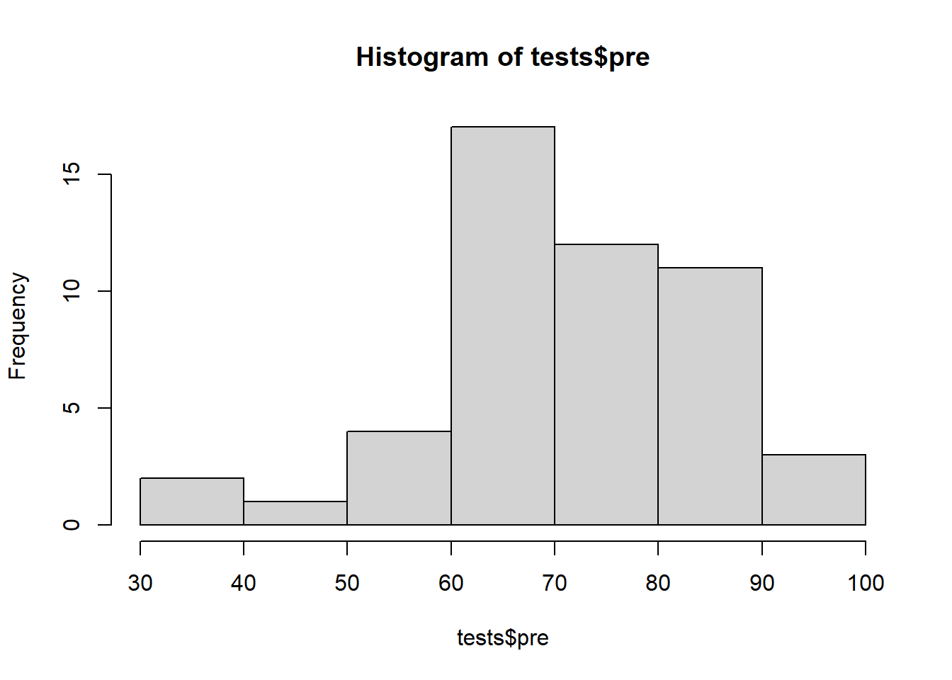

Above, the pre-test data looks like it might be normal but it isn’t very clear. The histogram makes it look like there are more observations above the mean than below the mean. Let’s continue checking for normality in different ways to see if we can get a more definitive answer.

The next method is to make what is called a quantile-quantile normal plot, or QQ plot for short.

Run the code below to make this plot:⁶¹

if (!require(car)) install.packages('car')
library(car)

qqPlot(tests$pre)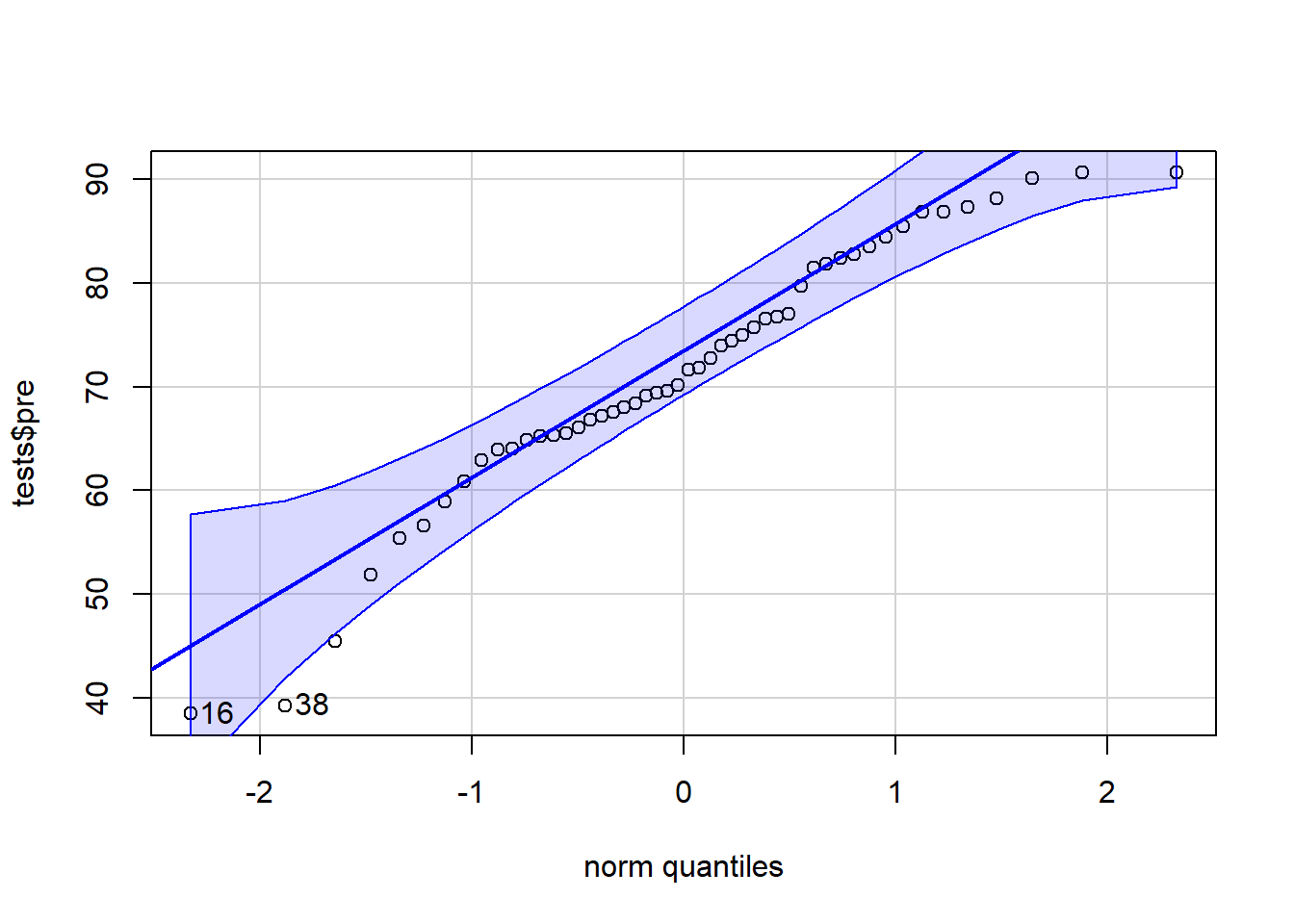

## [1] 16 38

In the code above, we gave our variable of interest—tests$pre—into the qqPlot(...) function from the car package. It then produced a QQ plot for us. A QQ plot plots our data on the y-axis against theoretical normal distribution quantiles on the x-axis. It is not required for you to fully understand the process by which the graph is created. It is most important for you to know how to interpret the graph.

If your data is perfectly normally distributed, your data points will all fall along the solid blue line. Of course, some deviation from this line is acceptable. Confidence bands have been drawn in dotted blue lines. If your data falls within these bands, there is a high chance that they were drawn from a normal distribution. If any data points fall outside of these bands, you might want to consider either removing those observations from your analysis or trying a test other than a t-test.

Now that we have covered two visual ways to inspect your data for normality, there is a third way that is non-visual and uses a hypothesis test to check for normality. This is called the Shapiro-Wilk normality test.

These are the hypotheses for the Shapiro-Wilk normality test:

$H_0$: The data are normally distributed.
$H_A$: The data are not normally distributed.

And here is the code to run the test:

shapiro.test(tests$pre)

## 
##  Shapiro-Wilk normality test
## 
## data:  tests$pre
## W = 0.95465, p-value = 0.05311

Above, we gave the tests$pre variable to the shapiro.test(...) function and it ran the test on our data.

We interpret this test using the p-value, which in this case is just above 0.05. This means that there is approximately 95% support for the alternate hypothesis, which in this case is that the data is not normally distributed. This evidence is strong enough to at least suggest that our data might not be normal. Therefore, in this case, our data might violate the normality assumption of the t-test. Therefore, we should not use a t-test on this data and we should not trust the results given by any t-tests which used this data.

If the p-value had been higher and the visual inspection methods had also made the data look more normal, then we would have been fine. But as it stands right now, we might not be. One solution could be to remove a few outliers and re-run our t-test. And another could simply be to use a different type of test to answer our question.

3.3.3.3 Homogeneity of variances

The third assumption that must be satisfied is that the variance of the two samples being compared in the t-test should have approximately the same variance as each other. This is required for only the independent samples t-test, not the paired sample t-test.

Let’s reload our data from our independent t-test that we ran earlier in this chapter, which tested the hypothesis about blood pressure medication.

This code loads the data:

treatment <- c(-8, -14.8, -6.8, -11.6, -10.2, -11.6, -4.8, -6.5, -9.9, -17.2, -10.7, -11.9, -8.7, -11.6, -8.6, -8.3, -10.9, -14.1, -8.8, -12.4, -14.1, -16.8, -1.8, -10.8, -15.1, -8.5, -11.2, -9.8, -10.9, -12.8, -9.2, -10.1, -12.2, -8.8, -8.5, -7.5, -10.2, -6.2, -11.4, -8.1, -15.3, -6.3, -7.2, -5.9, -13.4, -16.8, -10.7, -10.9, -12.9, -13.1)

control <- c(0, -3.5, -2.6, 3.7, -1.1, -0.6, -0.3, -1.5, 4.9, -1.8, -0.3, 0.2, -0.6, -6, -4.1, -0.5, -2.6, 0.4, 0.5, 1.9, -1, -0.1, 1.6, -3.2, -1, -3.7, 1.8, -4.2, 1, -2.2, 2, 5.5, 1.5, 1, 3.7, -1.5, -3.3, -2.7, -4.3, -7, -1.4, 5.2, 3.8, 4.6, -1.5, 2.1, -5.1, 0.5, 3.5, -0.7)

bpdata <- data.frame(group = rep(c("T", "C"), each = 50), SysBPChange = c(treatment,control))

Now that we have the bpdata dataset loaded once again, we can test to see if the treatment and control groups in this data have homogenous variances (meaning similar variances as each other).

We will ask R to run a hypothesis test for us to test for homogeneity of variances. These are the hypotheses for this test:

$H_0$: The two samples of data do have similar variances.
$H_A$: The two samples of data do not have similar variances.

To conduct this hypothesis test, we will use the following code:

var.test(SysBPChange ~ group, data = bpdata)

## 
##  F test to compare two variances
## 
## data:  SysBPChange by group
## F = 0.83685, num df = 49, denom df = 49, p-value = 0.5354
## alternative hypothesis: true ratio of variances is not equal to 1
## 95 percent confidence interval:
##  0.4748926 1.4746881
## sample estimates:
## ratio of variances 
##          0.8368504

Here’s what the code above asked the computer to do:

var.test(...) – Run the var.test(...) function, which runs what is called an F-test for homogeneity of variances.
SysBPChange ~ group – The data we want to check for homogeneity of variances is in the dependent variable SysBPChange and this data is divided up into two groups according to the group variable.
data = bpdata – The variables used in this test come from the dataset called bpdata.

We will evaluate the results of this hypothesis test by looking at the p-value, which in this case is approximately 0.54. This is a very high p-value, allowing us to easily fail to reject the null hypothesis. This means that we did not find evidence that our two samples for our t-test violate the homogeneity of variances assumption.

If this p-value had been closer to or lower than 0.05, then we would be concerned and we would have to consider using a different test to analyze our data.

3.3.3.4 Summary of assumptions for independent and paired t-tests

Here is a summary of which assumptions need to be tested using diagnostic tests for each type of t-test.

Independent samples t-test

Independence of observations
Normality of samples (and underlying populations; each of your two samples on their own need to be normally distributed, so you will run normality tests separately for each sample)
Homogeneity of variances (equal variances)

Paired sample t-test

Independence of observations (partially)
Normality of samples (and underlying populations)

3.3.3.5 When assumptions are not met

You may have noticed that in the paragraphs above, when our data violates or comes close to violating one of the t-test assumptions, you are told that you might want to use a different type of test. But what type of test would you use instead of a t-test? Here are some—though certainly not close to all—possibilities:

Wilcoxon Signed Rank test. This is used in similar situations as when a t-test is used, but the assumptions are less restrictive. If you have data that is well suited for a t-test but violates one or more t-test assumptions, the Wilcoxon Signed Rank test could be a simple solution. Run the command ?wilcox.test in R to learn more about this test. The implementation and interpretation of this test is fairly similar to those of a t-test. Both independent and paired varieties of this test are available.
Linear regression. We will learn about linear regression soon in this textbook. Linear regression is one of the most versatile and commonly used quantitative analysis methods and is often useful in situations where a t-test might otherwise be used.
Multilevel linear regression model (linear fixed effects or random effects model). We will learn about these types of models later in this textbook. These are types of linear regression models that are specifically designed to correct for situations in which standard test assumptions have been violated.

You have now reached the end of the new content in this chapter. You are ready to move on to this week’s assignment!

3.3.4 Optional videos about t-test theory and calculation

The contents of this section are not required for this course. They are completely optional. Below, you will find some videos about the statistical theory behind t-tests as well as a few examples that show exactly how a t-test is calculated. It is not required for you to know this theory or these calculation procedures. Our focus is on how to responsibly/cautiously calculate and interpret the results of a t-test, because that is all we have time for in this course.

We will begin by watching the following video, which explains the relationship between hypothesis testing and t-tests:⁶²

The video above can be viewed externally at https://www.youtube.com/watch?v=0zZYBALbZgg.

Next, have a look at this video that uses a single example to show the purpose of a t-test:⁶³

The video above can be viewed externally at https://www.youtube.com/watch?v=N2dYGnZ70X0.

In the video below, you can see an example of a t-test being conducted, including how it can be done in a spreadsheet software and calculated by hand. You are not required to learn how to conduct a t-test in a spreadsheet software or by hand. Here is the video:⁶⁴

The video above can be viewed externally at https://www.youtube.com/watch?v=pTmLQvMM-1M.

And this video goes through two examples in careful detail (much more than you are required to learn for our course):⁶⁵

The video above can be viewed externally at https://youtu.be/UcZwyzwWU7o.

3.4 Assignment

This assignment requires you to review and brainstorm about multiple types of hypothesis tests and quantitative research designs. You will then practice running and interpreting the results of independent and paired t-tests.

Please use a new RMarkdown file to complete this assignment and then submit your work as a knitted HTML, PDF, or DOCX file that was created from your RMarkdown file.

Remember that you can use your own data for the assignments in this course. You are not required to use the provided data. Feel free to discuss this with Anshul as necessary. You can also use your own data without asking first as long as you can accomplish all of the tasks with that data.

3.4.1 Inference and hypothesis tests

In this portion of the assignment, you will practice applying the logic of inference and hypothesis testing while also using your quantitative research design skills.

Task 1: Use your imagination to come up with your own example of a quantitative study that would require the use of inference and hypothesis testing. Be sure to clearly describe and specify the following items in your answer: question of interest, population of interest, sample, inference, inference procedure, unit of observation, null hypothesis, alternate hypothesis. Then, explain how you would evaluate the results of your hypothesis test, using the terms effect size, confidence interval, and p-value.

3.4.2 Independent samples t-test

In this part of the assignment, you will practice running an independent samples t-test. Imagine that we, some researchers, are trying to answer the following research question: How does fertilizer affect plant growth in the entire population of plants?

We conduct a randomized controlled trial in which some plants are given a fixed amount of fertilizer (treatment group) and other plants are given no fertilizer (control group). Then we measure how much each plant grows over the course of a month. Let’s say we have ten plants in each group and we find the following amounts of growth.

The 10 plants in the control group each grew this much, in inches (each number corresponds to one plant’s growth):

3.8641111
4.1185322
2.6598828
0.3559656
2.8639095
0.9020122
5.0527020
2.3293899
3.5117162
4.3417785

The 10 plants in the treatment group each grew this much, in inches:

7.532292
1.445972
6.875600
6.518691
1.193905
4.659153
3.512655
4.578366
8.791810
4.891557

Please load this data into R by copying the following code into your own file on your computer:

control <- c(3.8641111,4.1185322,2.6598828,0.3559656,2.8639095,0.9020122,5.0527020,2.3293899,3.5117162,4.3417785)
treatment <- c(7.532292,1.445972,6.875600,6.518691,1.193905,4.659153,3.512655,4.578366,8.791810,4.891557)

my_data <- data.frame( 
                group = rep(c("control", "treatment"), each = 10),
                growth = c(control, treatment)
                )

Above, you are creating a dataset called my_data which contains the plant growth data from our fertilizer experiment. Inspect the data in RStudio on your computer to make sure it looks the same as the listed growth data for the treatment and control groups above (before the code was provided).

You will run an independent samples t-test on this data to answer the research question.

Task 2: Present a standardized dataset description for the dataset my_data that you are using in this portion of the assignment.

Task 3: Create a boxplot to visualize any possible differences in growth in the two experimental groups.

Task 4: Write precisely-worded null and alternate hypotheses for your t-test.

Task 5: Are the null and alternate hypotheses that you just wrote about your sample of 20 plants or the entire population of plants that this sample represents?

Task 6: Run a t-test to test your hypotheses. Interpret the results carefully and draw a conclusion.

Task 7: Is the p-value telling you information about your sample or the entire population?

Task 8: Identify which diagnostic tests of assumptions apply to this t-test and evaluate/run all of them. Be very thorough, using both visual and numeric methods as applicable. Show both your R code, R output, and your thorough explanations of each test.

Task 9: Write a short final conclusion about the extent to which you can answer the research question.

3.4.3 Paired sample t-test

In this part of the assignment, you will practice running a paired sample t-test. Imagine that we, some researchers, are trying to answer the following research question: Is daily weightlifting exercise associated with a change in ability to lift weight?

To answer this question, we created a study with 100 subjects. On the first day, we measured how many squats each participant could do in one minute while wearing a ten pound vest (called pre data). We then had each participant participate in an exercise program for a month. At the end of that month, we again measured how many squats each participant could do in one minute while wearing a ten pound vest (called post data).

Use the code below to load this data into R:

pre <- c(6.9, 4.8, 16.4, 19.8, 16.2, 21.1, 15, 14.9, 9.4, 16.5, 21.6, 19.3, 7.1, 31.7, 24.7, 9.8, 19.1, 3.3, 15.4, 17.9, 18.2, 19, 6.4, 3.7, 24.5, 15.9, 9.6, 29.9, 18.2, 30.6, 22.4, 21.7, 6.5, 1.4, 28.9, 13.9, 7.6, 12.9, 17, 35.8, 23.1, 14.9, 18.3, -0.1, 7.4, 10.6, 21.7, 4.1, 9.1, -1.9, 32, 3.9, 30.3, 23.5, 23.6, 21, 9, 29.6, 12, 15.6, 11.4, 11.3, 35.4, 20.1, 10.1, 15.2, 6.3, 14.3, 29.2, 15.5, 8.3, -8.2, 4.5, 11.7, 14.1, -1.2, 23.9, 10.7, 23.8, 17.2, 25.6, 8.4, 12.7, 15, 15.8, 34.4, 30, 19.6, 23, 13.2, 1, 31.7, 18.9, -1.5, 30.2, 8.8, 27.2, 22.5, 27, 8.8)

post <- c(18.3, 13.4, 5.1, 8.4, 8.6, 26.2, 26.2, 21, 14, 9.1, 21.7, 9.5, 25.9, 26.7, 8.9, 9.4, 14.9, 13.6, 29.2, 10.4, 13.3, 18.4, 8, 8.2, 5.3, 27.7, 18.9, -0.9, 22, 11.5, 4.3, 26.9, 30, 13.6, 22, 15.4, 8.7, 11.7, 33, 31.3, 21.6, 25.7, 15.3, 17, 10, 32.8, 26.4, 19.4, 15.3, 25.4, 22.6, 10, 17.4, 27.9, 26, 24.7, 16.1, 21.3, 22, 5.6, 14.7, 23, 23.3, 31.1, 21.3, 24.5, 12.6, 13.9, 18.7, 18.5, 10, 17.5, 20.6, 22, 19.4, 14.3, 15.5, 12, 19.4, 15, 22.8, 9.2, 22.4, 22.9, 16.3, 23.2, 28.8, 15.3, 18, 13.6, 25.8, 28.7, 19.7, 17.5, 14.8, 9.5, 16, 29.1, 11.1, 18.2)

exercise <- data.frame(pre,post)

You now have a dataset called exercise that you will use for this part of the assignment. exercise contains two variables: pre and post.

Task 10: Instead of asking you to follow particular steps, now you will choose which steps you need to follow to responsibly conduct a complete analysis to answer this research question about exercise. You can use the content in this chapter and your own work in the previous portion of this assignment to guide you. Provide all descriptive statistics, inferential tests, interpretations, and diagnostic tests necessary to answer the question. You can ask instructors and each other for help along the way.

3.4.4 Practice with t-test results

In this part of the assignment, you will practice the skills of consuming, interpreting, and evaluating scholarship that has been conducted by others. Practicing and developing these skills can assist you, for example, in the following scenarios:

You need to evaluate the strengths and limitations of somebody else’s work, to determine how trustworthy their findings are.
You need to understand what somebody else’s research found, so that you understand how your own research relates to it.
You are collaborating with a statistician who is assisting you with an analysis. They present their results to you and you need to be able to understand these results, determine on your own if the statistician made any mistakes, and give appropriate feedback to the statistician.
You are asked to be a peer reviewer for a journal article that uses quantitative research methods.

To get started, read ONLY the abstract of the following article (DO NOT read the entire article):

Kim S, Willett LR, Pan WJ, Afran J, Walker JA, Shea JA. Impact of required versus self-directed use of virtual patient cases on clerkship performance: a mixed-methods study. Academic Medicine. 2018 May 1;93(5):742-9. https://doi.org/10.1097/ACM.0000000000001961.

It is important that you develop the ability to understand the details of a quantitative analysis from only reading a summary of it. This is why you should ONLY read the abstract portion of the article cited above.

Please complete the following tasks related to the Kim et al (2018) article, to the extent that ONLY the abstract allows you to do:

Task 11: What research question is being answered? Your answer should be a single sentence with a question mark at the end. It should mention the two experimental conditions being compared in the study.

Task 12: What type of t-test did the researchers use to answer their research question? Why did they use this kind of t-test? Even though they don’t explicitly say which type of t-test they used, you can figure it out from the description of the study in the abstract.

Task 13: For the outcome called “number of cases completed” for only the family medicine students, carefully state the hypothesis test that was conducted and write the null and alternate hypotheses.

Task 14: For the outcome called “number of cases completed” for only the family medicine students, what is the result of the t-test? Which experimental condition was better? Make sure your answer addresses the hypothesis test that you wrote earlier.

Now we will continue our practice of interpreting t-test results. Please read ONLY the abstract of the following article:

Heidemann LA, Keilin CA, Santen SA, Fitzgerald JT, Zaidi NL, Whitman L, Jones EK, Lypson ML, Morgan HK. Does performance on evidence-based medicine and urgent clinical scenarios assessments deteriorate during the fourth year of medical school? Findings from one institution. Academic Medicine. 2019 May 1;94(5):731-7. https://doi.org/10.1097/ACM.0000000000002583.

Please complete the following tasks related to the Heidemann et al (2019) article, to the extent that ONLY the abstract allows you to do:

Task 15: What research question is being answered? Your answer should be a single sentence with a question mark at the end.

Task 16: What type of t-test did the researchers use to answer their research question? Why did they use this kind of t-test?

Task 17: Which two outcomes did Heidemann et al look at?

Task 18: For the EBM outcome, what is the hypothesis test (describe what is being tested, null hypothesis, and alternate hypothesis).

Task 19: For the UCS outcome, what is the hypothesis test (describe what is being tested, null hypothesis, and alternate hypothesis).

Task 20: What is the result for the EBM outcome? Make sure your answer addresses the hypothesis test that you wrote earlier.

Task 21: What is the result for the UCS outcome? Make sure your answer addresses the hypothesis test that you wrote earlier.

3.4.5 Additional items

You have now reached the end of this week’s assignment. The tasks below will guide you through submission of the assignment, remind you of any other items you need to complete this week, and allow us to gather questions and/or feedback from you.

Task 22: You are required to complete 15 quiz question flashcards in the Adaptive Learner App by the end of this week.

Task 23: Please write any questions you have for the course instructors (optional).

Task 24: Please write any feedback you have about the instructional materials (optional).

Task 25: Knit (export) your RMarkdown file into an HTML, Word, or PDF file, as demonstrated earlier in the chapter. This knitted file is the one that you will submit.

Task 26: Please submit your assignment to the D2L assignment drop-box corresponding to this chapter and week of the course. Please e-mail all instructors if you experience any difficulty with this process. If you have trouble getting your RMarkdown file to knit, you can submit your RMarkdown file (instead of an HTML, Word, or PDF file).

Also called dependent sample t-test.↩︎
As you continue the course, you will learn a variety of methods for comparing the results of different inference procedures and deciding which ones to trust and not trust.↩︎
An athlete who tries to jump over bars to see how high of a bar they can jump over.↩︎
The reason for which we don’t have evidence doesn’t matter. It could be because Weeda attempted to jump and could not do it or because Weeda never attempted to jump. We just don’t have evidence that Weeda can do it.↩︎
Remember: our sample is the data spreadsheet that we have. If we have data on 100 people, our “sample” refers to just those 100 people. That sample of 100 people is drawn from a population (of many more than 100 people). We use inferential statistics, like p-values, to answer the hypothesis test for our population. For our sample of 100 people alone, we don’t need inferential statistics; we already know the truth in our sample so we don’t need to make guesses.↩︎
This particular bullet is a little oversimplified. In a two-sample (whether independent or paired) t-test for example, the t-test is helping us determine if the two samples come from different populations. Occasionally, maybe they don’t come from separate populations, but the p-value is still low and we reject the null hypothesis. But in this scenario, maybe the individuals we sampled just happened to make it seem like there is a difference in the two samples. That sampling was due to random chance. So the p-value in this example also tells us the probability that an outcome occurred due to random chance rather than the two samples actually being different from one another. It is not necessary to understand this explanation yet, especially since you won’t learn about t-tests until later.↩︎
This is a variety of between-subjects research design.↩︎
This is technically called a vector in R.↩︎
This is technically called a data frame in R↩︎
In this code, we did not give our data to the computer using a dataset. Instead, we gave the computer the outcome variable data for our two samples—treatment and control—separately, separated by a comma within the parentheses.↩︎
The test output reports: p-value < 2.2e-16. 2.2e-16 means $2.2*10^{-16} = 0.00000000000000022$, which is a very small number! This is telling us that there is an extremely small chance that rejecting the null hypothesis would be a mistake.↩︎
9.5 has been added to all treatment observations, to make the difference in sample means 0.6 mmHg now instead of 10.1 mmHg as it was initially. This mimics a situation in which the blood pressure medication did not help much.↩︎
This is a variety of within-subjects research design.↩︎
This code could also just be hist(pre) since pre also exists in our data on its own as a column of data that is not inside of a dataset. To make a histogram of treatment and control groups from our blood pressure example, you can run hist(treatment) and hist(control), without using the dataset bpdata as part of the command, since treatment and control are also loaded on your computer as separate columns of data that are not associated with a dataset.↩︎
This code could also just be qqPlot(pre) since pre also exists in our data on its own as a column of data that is not inside of a dataset. To make a histogram of treatment and control groups from our blood pressure example, you can run qqPlot(treatment) and qqPlot(control), without using the dataset bpdata as part of the command, since treatment and control are also loaded on your computer as separate columns of data that are not associated with a dataset.↩︎
Hypothesis testing: step-by-step, p-value, t-test for difference of two means - Statistics Help. Dr Nic’s Maths and Stats. Dec 5, 2011. YouTube. https://www.youtube.com/watch?v=0zZYBALbZgg.↩︎
What is a t-test?. U of G Library. Oct 23, 2017. YouTube. https://www.youtube.com/watch?v=N2dYGnZ70X0.↩︎
Student’s t-test. Bozeman Science. Apr 13, 2016. YouTube. https://www.youtube.com/watch?v=pTmLQvMM-1M.↩︎
Hypothesis Testing - Difference of Two Means - Student’s -Distribution & Normal Distribution. The Organic Chemistry Tutor. Nov 14, 2019. YouTube. https://youtu.be/UcZwyzwWU7o.↩︎