Chapter 4 Correlation and Simple OLS Linear Regression

This week, our goals are to…

Calculate and interpret a correlation coefficient to examine how related two variables (columns of data) are to each other.
Review the process that OLS linear regression uses to draw a line of best fit.
Run a simple OLS linear regression in R and interpret its coefficient estimates.
Interpret goodness-of-fit metrics for OLS linear regression.
Relate $R^2$ with correlation coefficient.
Use a dummy (binary) variable in a regression model.

Announcements and reminders

Like always, I suggest that you look at this week’s assignment first, before you read the chapter. You can even do the assignment while you read the chapter.
This week’s content requires you to recall details about linear relationships that you learned in an earlier week of the course.

4.1 Correlation

Correlation is a basic statistic that we can use to determine the relationship between two variables. A correlation coefficient—commonly written as $r$—gives a quantitative measure of how strongly related two variables are or are not. When we discuss correlation in this section, we will imagine that we are interested in the relationship between two variables, X and Y. X and Y can be negatively, zero, or positively correlated.

Here are what these three types of correlations mean:

Negative Correlation: As variable X increases, variable Y decreases
Zero Correlation: As variable X increases, we do not know what happens to variable Y.
Positive Correlation: As variable X increases, variable Y increases

The most common way in which correlation is calculated is called Pearson’s correlation or Pearson’s r. When we use correlation in this book, it will always refer to Pearson’s correlation unless otherwise specified. The terms r, correlation, and correlation coefficient are often used interchangeably; they all mean the same thing.

The correlation coefficient can range from -1 to +1.⁶⁶

-1 means that there is a perfect negative relationship between X and Y.
0 means that there is no relationship between X and Y.
+1 means that there is a perfect positive relationship between X and Y.

Here are some examples of correlation:⁶⁷

Unit of observation cities	X variable distance from ocean	Y variable flood incidents	Correlation -0.3	What it means cities with high distances from the ocean have fewer flood incidents

humans	age	distance from Havana	0	age is completely unrelated to how far from Havana people live
households	annual income	square footage of home	0.7	households with high annual incomes have homes with high square footages

Sometimes, we calculate the square of our correlation coefficient. This is often referred to as $R^2$, R-squared, R-square, or coefficient of determination. All of these terms mean the same thing. $R^2$ refers to the proportion (or percentage) of variation in Y that can be accounted for by variation in X. This statistic is commonly used alongside regression analysis.

4.1.1 Calculating and interpreting correlation – optional

Now that you have read a little bit about the concept of correlation, you may find it useful to see a few videos that demonstrate and apply the concept. It is completely optional (not required) for you to watch the videos in this section. Note that these videos were created by different instructor(s) for different audiences.

We’ll start with this video that gives an overview of correlation:⁶⁸

The video above can be viewed externally at https://www.youtube.com/watch?v=qC9_mohleao.

This follow-up video goes into more detail:⁶⁹

The video above can be viewed externally at https://www.youtube.com/watch?v=ugd4k3dC_8Y.

4.1.2 Correlation in R

Let’s turn to calculating correlation in R. To do this, we will just use the built-in dataset mtcars. Let’s create a dataset called d which is a copy of mtcars:

d <- mtcars

We can inspect our entire dataset d with the following command:

View(d)

In this example, we will just focus on the relationship between a car’s weight (wt) and displacement (disp). Keep in mind that each observation in our data set is a separate car (automobile). Note that weight is measured in tons and displacement is measured in cubic inches. Weight is our independent variable of interest and displacement is our dependent variable of interest.

Below, we can inspect our observations (cars) in our data just for these two variables of interest:⁷⁰

d[c("wt","disp")]

##                        wt  disp
## Mazda RX4           2.620 160.0
## Mazda RX4 Wag       2.875 160.0
## Datsun 710          2.320 108.0
## Hornet 4 Drive      3.215 258.0
## Hornet Sportabout   3.440 360.0
## Valiant             3.460 225.0
## Duster 360          3.570 360.0
## Merc 240D           3.190 146.7
## Merc 230            3.150 140.8
## Merc 280            3.440 167.6
## Merc 280C           3.440 167.6
## Merc 450SE          4.070 275.8
## Merc 450SL          3.730 275.8
## Merc 450SLC         3.780 275.8
## Cadillac Fleetwood  5.250 472.0
## Lincoln Continental 5.424 460.0
## Chrysler Imperial   5.345 440.0
## Fiat 128            2.200  78.7
## Honda Civic         1.615  75.7
## Toyota Corolla      1.835  71.1
## Toyota Corona       2.465 120.1
## Dodge Challenger    3.520 318.0
## AMC Javelin         3.435 304.0
## Camaro Z28          3.840 350.0
## Pontiac Firebird    3.845 400.0
## Fiat X1-9           1.935  79.0
## Porsche 914-2       2.140 120.3
## Lotus Europa        1.513  95.1
## Ford Pantera L      3.170 351.0
## Ferrari Dino        2.770 145.0
## Maserati Bora       3.570 301.0
## Volvo 142E          2.780 121.0

Next, let’s create a scatterplot of these two variables. We’ll put our outcome of interest on the vertical axis and our input of interest on the horizontal axis.

plot(d$wt, d$disp)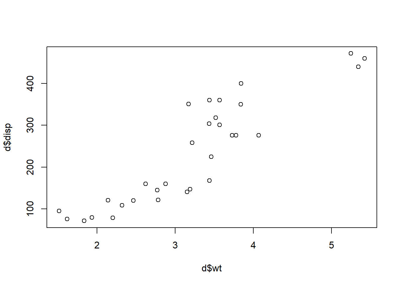

Just by visually inspecting the scatterplot above, you can see that there appears to be a close association between weight and displacement of a car in our sample. We are now ready to calculate the correlation of weight and displacement.

The code below calculates correlation in R:

cor(d$wt,d$disp)

## [1] 0.8879799

Here is what we asked the computer to do for us above:

cor(...) – Calculate the correlation between two variables, X and Y.
d$wt – X variable.
d$disp – Y variable.

As you can see, the correlation between weight and displacement is 0.89. This is a very high correlation. This means that cars with heavy weight are likely to also have high displacement.

We can save this calculated correlation in R’s memory in case we want to use it later:

r <- cor(d$wt,d$disp)

Above, we created the object r which saves the result of the code cor(d$wt,d$disp). You will notice that r now appears as a stored object within your environment in RStudio.

We can run the code r and the computer will show us that it did indeed store this for us:

## [1] 0.8879799

Above, we ran the command r and the computer responded to us by showing us that it stored 0.89 as r.

We can also calculate $R^2$ with the code below:

r^2

## [1] 0.7885083

Above, the computer is telling us that $R^2 = 0.79$, which is the square of 0.89.

You are now equipped to calculate and interpret correlations in R.

4.1.3 Correlation matrix in R

If we want to see correlations for multiple variables within a dataset all at once, we can create a correlation matrix. A correlation matrix can sometimes be large and difficult to read if we include all of the variables in a particular dataset in our matrix. A more straightforward approach is to create a separate dataset which includes only the variables for which you want to see correlations.

Here we make a partial dataset of mtcars called mtcars.partial:⁷¹

mtcars.partial <- mtcars[c("disp","wt","drat", "am")]

Our new dataset called mtcars.partial contains the variables disp, wt, drat, and am from our original mtcars dataset.

Now we can make a correlation matrix on the dataset mtcars.partial:

cor(mtcars.partial)

##            disp         wt       drat         am
## disp  1.0000000  0.8879799 -0.7102139 -0.5912270
## wt    0.8879799  1.0000000 -0.7124406 -0.6924953
## drat -0.7102139 -0.7124406  1.0000000  0.7127111
## am   -0.5912270 -0.6924953  0.7127111  1.0000000

In the output above, we see pairwise correlations for each combination of variables in our dataset. For example, disp and drat are correlated at -0.71.

A correlation matrix can help us quickly look for associations between variables in our data.

4.2 Ordinary least squares (OLS) line of best fit

One of the most important concepts that we will be learning and applying throughout this textbook is regression analysis. More specifically, linear regression is the most common form are for regression analysis that we will use. The purpose of linear regression is to fit a linear equation to a set of data.

You may recall that the most basic form of a linear equation can be written as $y=mx+b$ or $y=b_1x+b_0$. $m$ or $b_1$ refers to the slope of the line. $b$ or $b_0$ refers to the y-intercept of the line (the y-intercept can also be called just the intercept or the constant). For every one unit increase in X, Y increases by $m$ (or $b_1$) units. Remember that these words—“For every one unit increase in X”—are the magic words.

The most common type of linear regression is called OLS linear regression. OLS stands for ordinary least squares. This type of linear regression attempts to fit a line to our data that is as close to as many of the data points as possible. It uses the least squares method to fit the line. You will gain an intuition for the least squares method as you encounter the examples that follow in this chapter.

4.2.1 Videos about OLS

Below are a few videos that are optional (not required) for you to watch, if you feel that a few audio-visual examples might be useful. We will also walk through the steps and interpretation of linear regression later in the chapter. Some of these videos will give you a sense for how linear regression models are calculated and interpreted. Note that all of these videos were created by different instructors, for different audiences.

This video carefully walks through how a regression line is calculated:⁷²

The video above can be viewed externally at https://youtu.be/JvS2triCgOY.

And this video also demonstrates the calculation of the least squares regression line in a different way:⁷³

The video above can be viewed externally at https://www.youtube.com/watch?v=jEEJNz0RK4Q.

This video explains how we can analyze the extent to which there is error in a regression line, in addition to discussing regression more generally:⁷⁴

The video above can be viewed externally at https://www.youtube.com/watch?v=coQAAN4eY5s.

You will frequently have to interpret regression results that were produced by computer programs. The following video focuses on how to interpret these results:⁷⁵

The video above can be viewed externally at https://youtu.be/sIJj7Q77SVI.

4.2.2 OLS terminology

This sub-section is optional (not required) to read.

The popular drink Coca Cola can be referred to as “Coca Cola”, “Coke”, “Cola”, “soda”, “pop”, “soft drink”, and likely other terms too. But all of these terms mean the same thing; it’s just a difference in how people talk. Similarly, in this chapter and beyond, you might see terms like “regression”, “regression analysis”, “regression model”, “linear regression”, “OLS regression”, “OLS”, “OLS linear regression”, and maybe more used interchangeably. In our work together (and in most situations beyond that as well), all of these terms mean exactly the same thing. Regression analysis (often just called “regression”) is one of the main and most powerful quantitative analysis techniques for understanding the relationship between an independent and dependent variable. There are many different types of regression, and right now we are learning about the type of regression that we use when we suspect that our dependent and independent variable are linearly related to each other, which is where the term linear regression comes from. We will learn about other types of regression later.

The purpose of linear regression is to calculate a line or equation of best fit for our data. The most common process used to determine this line of best fit is a process called OLS (ordinary least squares). So that’s why you see the term OLS used alongside the terms “regression” and “linear regression”. Sometimes, someone might say “Let’s run OLS on this data,” which is just a brief way of saying: “Let’s run OLS linear regression on this data.” Someone might also say “Let’s run linear regression on this data,” which again usually is just shorthand for saying “Let’s run OLS linear regression on this data.” All of this is the same as saying “Let’s run an OLS linear regression analysis” or “Let’s run an OLS linear regression model”. The words “analysis” and “model” can be included or not; both ways are fine and the meaning is the same.

People who talk about Coca Cola a lot don’t say “I love the taste of the soft drink Coca Cola.” They say: “I love the taste of Coke.” Similarly, people who use OLS linear regression analysis models on a regular basis just say “I ran OLS.”

Right now, we are learning about how to analyze data in which there is just one dependent variable and just one independent variable. This is referred to as “simple” regression analysis or “bivariate” regression analysis (and of course people might also call this “simple OLS” or “bivariate OLS”; all of these terms mean exactly the same thing). Later on, we will learn how to analyze data with one dependent variable and more than one independent variables. We will never use regression analysis to analyze two or more dependent variables within a single analysis. We can have more than one independent variable but not more than one dependent variable. But again, that’s a topic for another day. Our focus right now is on analysis involving one dependent and one independent variable.

4.3 Simple OLS linear regression in R

In this section, we will run a simple OLS linear regression model in R and interpret the results. We will continue with the data and example that we used earlier in this chapter. Note that “simple” OLS regression refers to a regression analysis in which there is only one independent variable, which is the focus of this section. It is fine to refer to a regression model with one independent variable as a simple OLS linear regression, simple linear regression, OLS linear regression, or linear regression. All of these terms mean the same thing. The terms regression analysis and regression model can also be used interchangeably. They mean the same thing, for our purposes.

Here are the key details of the example regression analysis we will conduct:

Question: What is the association between displacement and weight in cars?
Dependent variable: disp; displacement in cubic inches.
Independent variable: wt; weight in tons.
Dataset: mtcars data in R, loaded as d in our example. Run the code d<-mtcars if you have not already, to load the data.

4.3.1 OLS in our sample

Let’s start by making a linear regression model on our sample with the R code below:

reg1 <- lm(disp~wt, data = d)

Here is what we are telling the computer to do with the code above:

reg1 – Create a new regression object called reg1. This can be named anything, not necessarily reg1.
<- – Assign reg1 to be the result of the output of the function lm(...)
lm(...) – Run a linear model using OLS linear regression.
disp – This is the dependent variable in the regression model.
~ – This is part of a formula. This is like the equals sign within an equation.
wt – This is the independent variable in the regression model.
data = d – Use the dataset d for this regression. d is where the dependent and independent variables are located.

If you look in the Environment tab in RStudio, you will see that reg1 is saved and listed there. Our regression results are stored as the object reg1 in R and we can refer back to them any time we want, as we will be doing multiple times below.

We are now ready to inspect the results of our regression model by using the summary(...) function to give us a summary of reg1, like this:

summary(reg1)

## 
## Call:
## lm(formula = disp ~ wt, data = d)
## 
## Residuals:
##    Min     1Q Median     3Q    Max 
## -88.18 -33.62 -10.05  35.15 125.59 
## 
## Coefficients:
##             Estimate Std. Error t value Pr(>|t|)    
## (Intercept)  -131.15      35.72  -3.672 0.000933 ***
## wt            112.48      10.64  10.576 1.22e-11 ***
## ---
## Signif. codes:  0 '***' 0.001 '**' 0.01 '*' 0.05 '.' 0.1 ' ' 1
## 
## Residual standard error: 57.94 on 30 degrees of freedom
## Multiple R-squared:  0.7885, Adjusted R-squared:  0.7815 
## F-statistic: 111.8 on 1 and 30 DF,  p-value: 1.222e-11

Above, we see summary output of our regression model. The most important section that we will look at first is the Coefficients section of the output. In the linear equation $y=mx+b$, $m$ and $b$ are called coefficients. In the linear equation $y=b_1x+b_0$, $b_1$ and $b_0$ are called coefficients. For the rest of our work together, we will use the $y=b_1x+b_0$ version of the linear equation.

We learn the following details from the Coefficients section of the regression output:

$b_0 = -131.15$ – This means that the intercept⁷⁶ is -131.15.
$b_1 = 112.48$ – This means that the slope of wt is 112.48.

We can follow these steps to write this regression result as an equation:

Start with the generic form of the linear equation: $y=b_1x+b_0$
Replace $b_0$ and $b_1$ with the corresponding numbers from the regression output: $y=112.48x-131.15$
Replace $y$ and $x$ with the correct variable names from our dataset: $disp=112.48wt-131.15$
Add a hat to the dependent variable, to indicate that this equation calculates predicted values (rather than actual values) of the dependent variable: $\hat{disp}=112.48wt-131.15$

$\hat{disp}=112.48wt-131.15$ is the final equation. This equation defines the line that bests fits our data in our sample, according to the OLS linear regression method.

Now we can interpret these results by looking at the equation:

Slope of wt: For every one ton increase in weight, displacement is predicted to increase by 112.48 cubic inches in our sample.
Intercept: When weight is equal to 0 tons, the predicted value of displacement is -131.15 cubic inches in our sample. This prediction of a negative number doesn’t make sense, of course. We are typically more interested in knowing the slope rather than the intercept of a regression model, because the slope is typically going to be what helps us answer our question of interest.

You should always start with the magic words “For every one unit increase in X…” when you are interpreting regression results.

Note that we did NOT prove that the independent variable weight is causing the dependent variable displacement. We only found that there is an association between these two variables in our sample.

We can do a little bit of basic math on our regression equation to see that the slope and intercept above are correct. We do this by plugging hypothetical numbers into the regression equation. Let’s imagine a car that weighs 2 tons and that we want to use our regression equation to calculate the predicted displacement for this car. We do this by substituting the number 2 in place of $wt$ in our equation:

$\hat{disp}=112.48*2-131.15 = 93.81$

This means that our regression model predicts that when a car weighs 2 tons, it has a displacement of 93.81 cubic inches.

Below, we plug in a few different values for $wt$ in our equation $\hat{disp}=112.48wt-131.15$:

$wt$	Calculation	$\hat{disp}$	Interpretation
0	$\hat{disp}=112.48*0-131.15 = -131.15$	-131.15 cubic inches	When a car weighs 0 tons, it has a predicted displacement of -131.15 cubic inches. This is the intercept of our regression result. In this case, the intercept is not particularly meaningful, because there is no such thing as a car that weighs 0 tons.
1	$\hat{disp}=112.48*1-131.15 = -18.67$	-18.67 cubic inches	When a car weighs 1 ton, it has a predicted displacement of -18.67 cubic inches.
2	$\hat{disp}=112.48*2-131.15 = 93.81$	93.81 cubic inches	When a car weighs 2 tons, it has a predicted displacement of 93.81 cubic inches.
3	$\hat{disp}=112.48*3-131.15 = 206.29$	206.29 cubic inches	When a car weighs 3 tons, it has a predicted displacement of 206.29 cubic inches.

We can make the following observations about the table above:

When we change the weight from 0 to 1, the predicted displacement changes from -131.15 to -18.67. This change is a difference of $-18.67-(-131.15) = 112.48$.
When we change the weight from 1 to 2, the predicted displacement changes from -18.67 to 93.81. This change is a difference of $93.81-(-18.67) = 112.48$.
When we change the weight from 2 to 3, the predicted displacement changes from 93.81 to 206.29. This change is a difference of $206.29-93.81 = 112.48$.
We could keep going like this and we would always find that when we increase weight by one ton, predicted displacement would increase by 112.48.

The calculations above confirm that 112.48 cubic inches is the slope of the association between displacement and weight in our sample.

Our equation $\hat{disp}=112.48wt-131.15$ tells us the exact relationship on average between displacement and weight in our sample. Everything written above has pertained to our sample only. We will now turn our attention to inference and our population of interest.

4.3.2 OLS in our population

We are now interested in answering this question: What is the true relationship between displacement and weight in the population from which our sample was selected?

To answer this question, we have to look at some of the inferential statistics that are calculated when we do a regression analysis. We also need to conduct some diagnostic tests of assumptions before we can trust the results.

We will start by calculating the 95% confidence intervals for our estimated regression coefficients, by running the confint(...) function on our saved regression results—called reg1—like this:

confint(reg1)

##                 2.5 %   97.5 %
## (Intercept) -204.0914 -58.2054
## wt            90.7579 134.1984

It is also possible to create a regression summary table that contains everything we need all in one place, using the summ(...) function from the jtools package.

Run the following code to load the package and see our regression results:

if (!require(jtools)) install.packages('jtools')
library(jtools)

summ(reg1, confint = TRUE)

Observations	32
Dependent variable	disp
Type	OLS linear regression

F(1,30)	111.85
R²	0.79
Adj. R²	0.78

	Est.	2.5%	97.5%	t val.	p
(Intercept)	-131.15	-204.09	-58.21	-3.67	0.00
wt	112.48	90.76	134.20	10.58	0.00
Standard errors: OLS

Here is what the lines of code above accomplished:

if (!require(jtools)) install.packages('jtools') – Check if the jtools package is already installed and install it if not.
library(jtools) – Load the jtools package.
summ(reg1, confint = TRUE) – Create a summary output of the saved reg1 regression result. Include the confidence intervals (because confint is set to TRUE).

We can now interpret the 95% confidence intervals that were calculated:

Slope: In the population from which our sample was drawn, we are 95% confident that the slope of the relationship between displacement and weight is between 90.76 and 134.20 cubic inches. In other words: In our population of interest, we are 95% confident that for every one ton increase in a car’s weight, its displacement is predicted to increase by at least 90.76 cubic inches or at most 134.20 cubic inches. This is the answer to our question of interest, if our data passes all diagnostic tests that we will conduct later.
Intercept: In the population from which our sample was drawn, we are 95% confident that the intercept of the relationship between displacement and weight is between -204.09 and -58.21 cubic inches. In other words: In our population of interest, we are 95% confident that a car that weighs 0 tons has a displacement between -204.09 and -58.21 cubic inches. Of course, this intercept is not very meaningful to us (which is fine) because there is no such thing as a car that is weightless.

Note that we did NOT prove that the independent variable weight is causing the dependent variable displacement. We only found that there is potentially—not definitely—an association between these two variables in our population of interest.

The computer conducted a number of hypothesis tests for us when it ran our regression analysis. The most important of these hypothesis tests relates to the slope estimate for displacement and weight.

Here is the framework for this hypothesis test:

$H_0$: In the population of interest, $b_1 = 0$. In other words: in the population of interest, there is no relationship between displacement and weight of cars.
$H_A$: In the population of interest, $b_1 \ne 0$. In other words: in the population of interest, there is a non-zero relationship between displacement and weight of cars.

We find the result of this hypothesis test within the regression output. The p-value for weight is extremely small, listed as 0.00 in one summary table and 1.22e-11 in another. This means that we have very high confidence in the alternate hypothesis $H_A$, meaning that there likely is an association between displacement and weight in our population of interest. More specifically, we are 95% confident that the slope of the association between displacement and weight in the population is between 90.76 and 134.20 cubic inches. Taking the p-value and confidence intervals into consideration, we reject the null hypothesis.

Here are some important reminders about our OLS linear regression results:

All of the estimated coefficients are measured in units of the dependent variable.
The slope of 112.48 cubic inches is the true average relationship between displacement and weight in our sample alone.
The 95% confidence intervals and p-values pertain to the population.
The slope of 112.48 cubic inches is the midpoint of the 95% confidence interval.⁷⁷
None of these results for the population of interest can be trusted until certain diagnostic tests of assumptions have been conducted.

4.3.3 Graphing OLS results

We can also graph the results of our OLS regression on a scatterplot. And this scatterplot will help us visualize some key characteristics about our regression line.

To make the plot of our data points and regression line, run this code:

plot(d$wt,d$disp)
abline(reg1)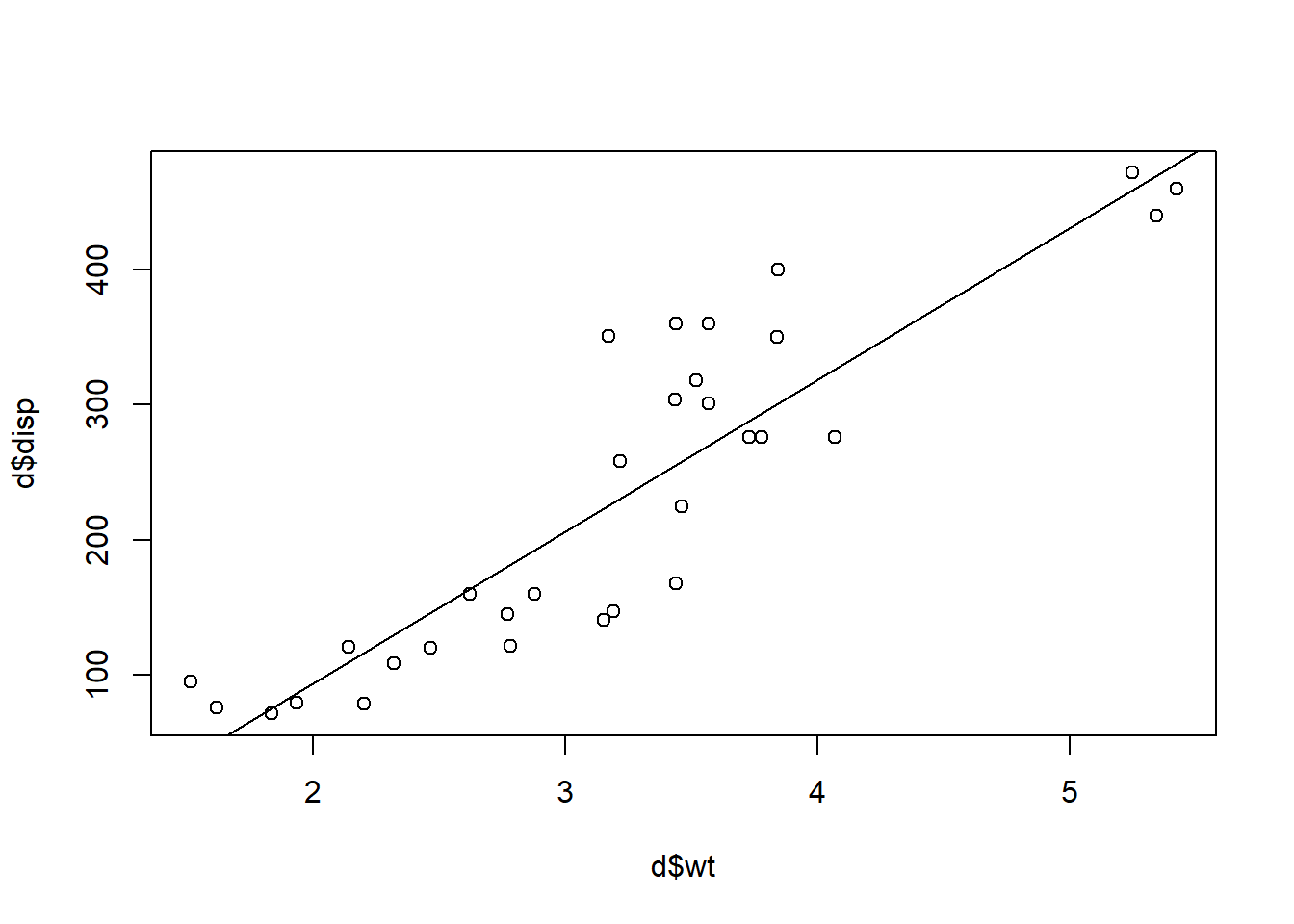

Here is what the code above asked the computer to do:

plot(d$wt,d$disp) – Create a scatterplot with d$wt on the horizontal axis and d$disp on the vertical axis.
abline(reg1, col = 'blue') – Add the regression line for reg1 to the already created scatterplot.

The scatterplot shows that the regression line fits the data pretty well. Most of the points are pretty close to the line. This means that there is not much error in the regression line. Such a well-fitting result is not common in social science, behavioral science, health, and education data.

4.3.4 Generic code for OLS linear regression in R

This section contains a generic version of the code and interpretation that you can use to run a simple OLS linear regression in R. You can copy the code below and follow the guidelines to replace elements of this code such that it is useful for analyzing your own data.

To run an OLS linear regression in R, you will use the lm(...) command:

reg1 <- lm(DepVar ~ IndVar, data = mydata)

Here is what we are telling the computer to do with the code above:

reg1 – Create a new regression object called reg1. You can call this whatever you want. It doesn’t need to be called reg1.
<- – Assign reg1 to be the result of the output of the function lm(...)
lm(...) – Run a linear model using OLS linear regression.
DepVar – This is the dependent variable in the regression model. You will write the name of your own dependent variable instead of DepVar.
~ – This is part of a formula. This is like the equals sign within an equation.
IndVar – This is the independent variable in the regression model. You will write the name of your own independent variable instead of IndVar.
data = mydata – Use the dataset mydata for this regression. mydata is where the dependent and independent variables are located. You will replace mydata with the name of your own dataset.

Then we would run the following command to see the results of our saved regression, reg1:

summary(reg1)

The summary(...) function shows you the results of the regression that you created and saved as reg1.

If you look in your Environment tab in RStudio, you will see that reg1 (or whatever you called your regression) is saved and listed there.

A summary table with confidence intervals can be created with the following code:

if (!require(jtools)) install.packages('jtools')
library(jtools)

summ(reg1, confint = TRUE)

4.4 OLS residuals

We will continue using the reg1 regression model that we created earlier in this chapter, which examined the relationship between displacement and weight of cars. Earlier in the chapter, our focus was on interpreting the slope and intercept in the regression model. Now we will turn our attention to an analysis of the individual observations in our dataset. Below, we will examine errors between our actual and predicted values of displacement in our regression model.

Remember: Displacement (disp) is our dependent variable and weight (wt) is our independent variable in this regression model. The dependent variable is our outcome of interest that we care about. Our main concern when we analyze residuals and error is our predictions of the dependent variable made by the regression model. Most of the procedure below is based on the dependent variable alone, which is displacement (disp).

Earlier in the chapter, we calculated predicted values of hypothetical cars that weighed 0, 1, 2, and 3 tons. We did this by plugging these numbers in for $weight$ into our regression equation $\hat{disp}=112.48wt-131.15$. Now we are going to plug the actual (real, not predicted) values of weight for the observations in our dataset and plug those into our regression equation. This process generates what is called the predicted values or fitted values of our regression model.⁷⁸

Here we calculate predicted values in R:

d$disp.predicted <- predict(reg1)

Here’s what the code above did:

d$disp.predicted <- – Create a new variable called disp.predicted within the dataset d. The new variable will be assigned the values of the code to the right of the <- operator.
predict(reg1) – Calculate predicted values for the regression model reg1.

Now a new variable called disp.predicted has been added to our dataset d. You can inspect this new variable by opening d in R on your own computer, using the View(...) command:

View(d)

In the table below, you can see our independent variable (wt), dependent variable (disp), and predicted values of the dependent variable (disp.predicted).

d[c("wt","disp","disp.predicted")]

##                        wt  disp disp.predicted
## Mazda RX4           2.620 160.0      163.54431
## Mazda RX4 Wag       2.875 160.0      192.22623
## Datsun 710          2.320 108.0      129.80087
## Hornet 4 Drive      3.215 258.0      230.46880
## Hornet Sportabout   3.440 360.0      255.77638
## Valiant             3.460 225.0      258.02594
## Duster 360          3.570 360.0      270.39854
## Merc 240D           3.190 146.7      227.65685
## Merc 230            3.150 140.8      223.15772
## Merc 280            3.440 167.6      255.77638
## Merc 280C           3.440 167.6      255.77638
## Merc 450SE          4.070 275.8      326.63761
## Merc 450SL          3.730 275.8      288.39504
## Merc 450SLC         3.780 275.8      294.01895
## Cadillac Fleetwood  5.250 472.0      459.36181
## Lincoln Continental 5.424 460.0      478.93301
## Chrysler Imperial   5.345 440.0      470.04723
## Fiat 128            2.200  78.7      116.30349
## Honda Civic         1.615  75.7       50.50378
## Toyota Corolla      1.835  71.1       75.24897
## Toyota Corona       2.465 120.1      146.11020
## Dodge Challenger    3.520 318.0      264.77463
## AMC Javelin         3.435 304.0      255.21399
## Camaro Z28          3.840 350.0      300.76764
## Pontiac Firebird    3.845 400.0      301.33003
## Fiat X1-9           1.935  79.0       86.49678
## Porsche 914-2       2.140 120.3      109.55480
## Lotus Europa        1.513  95.1       39.03101
## Ford Pantera L      3.170 351.0      225.40728
## Ferrari Dino        2.770 145.0      180.41603
## Maserati Bora       3.570 301.0      270.39854
## Volvo 142E          2.780 121.0      181.54081

In the table above, the final observation is a car called the Volvo 142E. Let’s use this car as an example to see how the computer calculated the predicted value for the Volvo 142E.

Procedure for calculating predicted displacement (dependent variable) for Volvo 142E:

Start with regression equation: $\hat{disp}=112.48wt-131.15$
See that the Volvo 142E weighs 2.780 tons.
Plug 2.780 tons into the regression equation: $\hat{disp}=112.48*2.780-131.15 = 181.54 cubic inches$
The predicted displacement from our regression model of the Volvo 142E is 181.54 cubic inches.

Here is what we know about the Volvo 142E:

Weight: $wt = 2.780\text{ tons}$. This is how much the Volvo 142E truly weighs in reality.
Actual displacement: $disp = 121.0\text{ cubic inches}$. This is how much displacement the Volvo 142E truly has in reality.
Predicted displacement: $\hat{disp} = 181.54\text{ cubic inches}$. This is how much displacement the regression model “thinks” the Volvo 142E has.

Remember that you saw the scatterplot of the data points and the regression line. In that scatterplot, there was some distance between the points and the line in most cases. We are now about to calculate the distances between the points and the line.

For the Volvo 142E, the actual value (the plotted point) of disp—called $disp$—is 121.0 cubic inches; and the predicted value from the regression equation of disp—called $\hat{disp}$—is 181.54 cubic inches. This means that there is some error.

Here are a few ways to write the error:

$Error = Actual - Predicted = 121.0 - 181.54 = -60.54$
$\epsilon = disp - \hat{disp} = 121.0 - 181.54 = -60.54$

Above, $\epsilon$ means error. $disp$ means actual value of displacement. $\hat{disp}$ means predicted value of displacement. The hat over a variable’s name means that it is a predicted value. Notice that this analysis of error so far has related to the dependent variable (our outcome of interest). We calculate errors for the dependent variable only.

The error for the Volvo 142E is -60.54. This is called the residual for the Volvo 142E. Our goal in OLS linear regression is to make a line for which the residual values for all of the observations are—overall—as low as possible. Now we will calculate and analyze the residuals for all of the observations in the data. The terms, residual values, residuals, and residual errors can all be used to mean the same thing, in the context of regression.

We run the following code to calculate the regression residuals:

d$disp.resid <- resid(reg1)

Here’s what we asked the computer to do with the code above:

d$disp.resid <- – Create a new variable called disp.resid within the dataset d. The new variable will be assigned the values of the code to the right of the <- operator.
resid(reg1) – Calculate residual values for the regression model reg1.

Now a new variable called disp.resid has been added to our dataset d. You can inspect this new variable by opening d in R on your own computer, using the View(...) command:

View(d)

In the table below, you can see our independent variable (wt), dependent variable (disp), predicted values of the dependent variable (disp.predicted), and the residuals (disp.resid):

d[c("wt","disp","disp.predicted","disp.resid")]

##                        wt  disp disp.predicted disp.resid
## Mazda RX4           2.620 160.0      163.54431  -3.544307
## Mazda RX4 Wag       2.875 160.0      192.22623 -32.226232
## Datsun 710          2.320 108.0      129.80087 -21.800865
## Hornet 4 Drive      3.215 258.0      230.46880  27.531201
## Hornet Sportabout   3.440 360.0      255.77638 104.223620
## Valiant             3.460 225.0      258.02594 -33.025943
## Duster 360          3.570 360.0      270.39854  89.601462
## Merc 240D           3.190 146.7      227.65685 -80.956846
## Merc 230            3.150 140.8      223.15772 -82.357720
## Merc 280            3.440 167.6      255.77638 -88.176380
## Merc 280C           3.440 167.6      255.77638 -88.176380
## Merc 450SE          4.070 275.8      326.63761 -50.837608
## Merc 450SL          3.730 275.8      288.39504 -12.595040
## Merc 450SLC         3.780 275.8      294.01895 -18.218947
## Cadillac Fleetwood  5.250 472.0      459.36181  12.638189
## Lincoln Continental 5.424 460.0      478.93301 -18.933007
## Chrysler Imperial   5.345 440.0      470.04723 -30.047234
## Fiat 128            2.200  78.7      116.30349 -37.603489
## Honda Civic         1.615  75.7       50.50378  25.196222
## Toyota Corolla      1.835  71.1       75.24897  -4.148968
## Toyota Corona       2.465 120.1      146.11020 -26.010195
## Dodge Challenger    3.520 318.0      264.77463  53.225369
## AMC Javelin         3.435 304.0      255.21399  48.786010
## Camaro Z28          3.840 350.0      300.76764  49.232364
## Pontiac Firebird    3.845 400.0      301.33003  98.669974
## Fiat X1-9           1.935  79.0       86.49678  -7.496782
## Porsche 914-2       2.140 120.3      109.55480  10.745200
## Lotus Europa        1.513  95.1       39.03101  56.068992
## Ford Pantera L      3.170 351.0      225.40728 125.592717
## Ferrari Dino        2.770 145.0      180.41603 -35.416028
## Maserati Bora       3.570 301.0      270.39854  30.601462
## Volvo 142E          2.780 121.0      181.54081 -60.540809

In the final row of the table above, you can see that the computer calculated the same residual value for the Volvo 142E that we had calculated ourselves, -60.54 cubic inches. The computer has also calculated for us the residual value of all observations. You can choose a few other observations and calculate for yourself. You will find that the residual is always the difference between the actual and predicted value for each observation.

The residuals in a regression analysis will be useful to us as we run a variety of analyses.

4.5 R-squared metric of goodness of fit in OLS

All regression models have a variety of goodness-of-fit measures that help us understand how well the entire⁷⁹ regression model fits our data and/or how appropriate it is for our data. In this section, we will learn about the measure called $R^2$. This measure is referred to as “R-squared”, “R-square”, “Multiple R-squared”, or something similar. They all mean the same thing.

If you look at the summary table that we made for reg1, you will see that it says Multiple R-squared: 0.7885. This number can also be interpreted as 78.9%. This means that 78.9% of the variation in the Y variable (disp) is accounted for by variation in the X variable (wt). This is a very high $R^2$ in the context of social science, behavioral, health, and education data. Every time you run an OLS regression (and many other types of regressions as well), you should examine the $R^2$ statistic to see how well your regression model fits your data.

The $R^2$ statistic tells us how well our independent variable helps us predict the value of our dependent variable. Our ultimate goal is to make good predictions of the dependent variable by fitting the best regression line possible to the data. Once you know the $R^2$ of a regression model, you can also use that to compare it to other regression models to see which model has the better fitting line. We will practice doing this later in this textbook.

Most importantly, keep the following in mind about $R^2$:

If $R^2$ is…	How is the model fit?	The residual errors are…	In a scatterplot with a regression line and plotted points…
high	good	small	The points are close to the line
low	bad	big	The points are far away from the line

$R^2$ has an interesting connection to correlation. $R^2$ is the square of the correlation of the actual and predicted values in any OLS linear regression. We will demonstrate this by calculating in R, below.

4.5.1 Correlation and R-squared

We have already calculated the predicted values from our regression model and added them to our dataset d. Below, we calculate the correlation coefficient of the actual and predicted values of disp in our dataset d.

Here we use the cor(...) function to correlate disp and disp.predicted:

cor(d$disp,d$disp.predicted)

## [1] 0.8879799

And we can also save this correlation as r.reg using this code:

r.reg <- cor(d$disp,d$disp.predicted)

Now r.reg is saved in R’s memory for us to use later if we want. You will see it listed in the environment.

Now we will calculate the square of r.reg:

r.reg^2

## [1] 0.7885083

Above, we see that this square of the correlation of actual and predicted values is the same as the $R^2$ metric from the OLS regression that we ran. Soon—not in this chapter, though—we will be adding more than one independent variable into our regression models. Even with more than one independent variable, the square of the correlation of the actual and predicted values will be equal to the $R^2$ statistic in an OLS linear regression.

Remember:

The actual values are the true outcome numbers that our independent variable and our regression model are attempting to guess (predict).
The predicted values are the best guesses (predictions) that the independent variable in our regression model is able to make about the actual values of the dependent variable. These predicted values represent the variation in the independent variable.
The correlation of the actual values (true outcomes) and predicted values (best guesses) tells us how well-fitting our regression model is.

4.5.2 Calculating R-squared

Now we will learn how exactly $R^2$ is calculated. To calculate $R^2$, we have to first calculate two values called SSR and SST:

SSR means sum of squares regression.
SST means sum of squares total.

First we will calculate SSR. We begin this process by calculating the squares of all residuals. We had already calculated residuals before, so we just need to create a new variable in our dataset d which is the square of the residuals.

Here is the code to square the residuals:

d$disp.resid2 <- d$disp.resid^2

Here is what the code above is doing:

d$disp.resid2 <- – Create a new variable called disp.resid2 within the dataset d. disp.resid2 will be equal to the value calculated by the code to the right of the <- operator.
d$disp.resid^2 – Square the value of disp.resid for each observation within the dataset d.

We can examine our dataset d with the added new variable disp.resid2—which stands for “displacement residual squared”—by running the View(...) function:

View(d)

Below is a table of d with the new disp.resid2 variable added:

d[c("wt","disp","disp.predicted","disp.resid","disp.resid2")]

##                        wt  disp disp.predicted disp.resid disp.resid2
## Mazda RX4           2.620 160.0      163.54431  -3.544307    12.56211
## Mazda RX4 Wag       2.875 160.0      192.22623 -32.226232  1038.53004
## Datsun 710          2.320 108.0      129.80087 -21.800865   475.27773
## Hornet 4 Drive      3.215 258.0      230.46880  27.531201   757.96702
## Hornet Sportabout   3.440 360.0      255.77638 104.223620 10862.56290
## Valiant             3.460 225.0      258.02594 -33.025943  1090.71292
## Duster 360          3.570 360.0      270.39854  89.601462  8028.42194
## Merc 240D           3.190 146.7      227.65685 -80.956846  6554.01087
## Merc 230            3.150 140.8      223.15772 -82.357720  6782.79408
## Merc 280            3.440 167.6      255.77638 -88.176380  7775.07405
## Merc 280C           3.440 167.6      255.77638 -88.176380  7775.07405
## Merc 450SE          4.070 275.8      326.63761 -50.837608  2584.46234
## Merc 450SL          3.730 275.8      288.39504 -12.595040   158.63504
## Merc 450SLC         3.780 275.8      294.01895 -18.218947   331.93004
## Cadillac Fleetwood  5.250 472.0      459.36181  12.638189   159.72383
## Lincoln Continental 5.424 460.0      478.93301 -18.933007   358.45875
## Chrysler Imperial   5.345 440.0      470.04723 -30.047234   902.83627
## Fiat 128            2.200  78.7      116.30349 -37.603489  1414.02236
## Honda Civic         1.615  75.7       50.50378  25.196222   634.84962
## Toyota Corolla      1.835  71.1       75.24897  -4.148968    17.21394
## Toyota Corona       2.465 120.1      146.11020 -26.010195   676.53026
## Dodge Challenger    3.520 318.0      264.77463  53.225369  2832.93986
## AMC Javelin         3.435 304.0      255.21399  48.786010  2380.07481
## Camaro Z28          3.840 350.0      300.76764  49.232364  2423.82570
## Pontiac Firebird    3.845 400.0      301.33003  98.669974  9735.76369
## Fiat X1-9           1.935  79.0       86.49678  -7.496782    56.20174
## Porsche 914-2       2.140 120.3      109.55480  10.745200   115.45931
## Lotus Europa        1.513  95.1       39.03101  56.068992  3143.73190
## Ford Pantera L      3.170 351.0      225.40728 125.592717 15773.53057
## Ferrari Dino        2.770 145.0      180.41603 -35.416028  1254.29501
## Maserati Bora       3.570 301.0      270.39854  30.601462   936.44946
## Volvo 142E          2.780 121.0      181.54081 -60.540809  3665.18955

Above, we see that for each observation, the value of disp.resid2 is the square of the value of disp.resid.

The next step as we continue to calculate SSR is to calculate the sum of the squared residuals column.

The code below sums up the disp.resid2 column:

sum(d$disp.resid2)

## [1] 100709.1

The sum above is the SSR. The SSR is the sum of all squared residuals. In this data, SSR = 100709.1

Now we will turn to calculating SST. The first step is to determine the mean of the dependent variable, disp.

We can use the mean(...) function to calculate this:

mean(d$disp)

## [1] 230.7219

The next step is to subtract the dependent variable’s value from the mean of the dependent variable for each observation.

This code subtracts the mean from each disp:

d$disp.meandiff <- d$disp-230.7219

Here is what we are asking the computer to do above:

d$disp.meandiff <- – Create a new variable called meandiff in the dataset d which will be equal to the calculated values by the code on the right side of the <- operator.
d$disp-230.7219 – For each observation in d, subtract 230.7219 (which is the mean of the variable disp) from that observation’s value of disp.

The next step is to square the meandiff variable:

d$disp.meandiff2 <- d$disp.meandiff^2

And now we can have a look at our data again. In R, run the View(…) command to inspect our dataset d with all of the new variables included:

View(d)

In the table below we see some of the recently added variables:

d[c("wt","disp","disp.resid","disp.resid2","disp.meandiff","disp.meandiff2")]

##                        wt  disp disp.resid disp.resid2 disp.meandiff
## Mazda RX4           2.620 160.0  -3.544307    12.56211      -70.7219
## Mazda RX4 Wag       2.875 160.0 -32.226232  1038.53004      -70.7219
## Datsun 710          2.320 108.0 -21.800865   475.27773     -122.7219
## Hornet 4 Drive      3.215 258.0  27.531201   757.96702       27.2781
## Hornet Sportabout   3.440 360.0 104.223620 10862.56290      129.2781
## Valiant             3.460 225.0 -33.025943  1090.71292       -5.7219
## Duster 360          3.570 360.0  89.601462  8028.42194      129.2781
## Merc 240D           3.190 146.7 -80.956846  6554.01087      -84.0219
## Merc 230            3.150 140.8 -82.357720  6782.79408      -89.9219
## Merc 280            3.440 167.6 -88.176380  7775.07405      -63.1219
## Merc 280C           3.440 167.6 -88.176380  7775.07405      -63.1219
## Merc 450SE          4.070 275.8 -50.837608  2584.46234       45.0781
## Merc 450SL          3.730 275.8 -12.595040   158.63504       45.0781
## Merc 450SLC         3.780 275.8 -18.218947   331.93004       45.0781
## Cadillac Fleetwood  5.250 472.0  12.638189   159.72383      241.2781
## Lincoln Continental 5.424 460.0 -18.933007   358.45875      229.2781
## Chrysler Imperial   5.345 440.0 -30.047234   902.83627      209.2781
## Fiat 128            2.200  78.7 -37.603489  1414.02236     -152.0219
## Honda Civic         1.615  75.7  25.196222   634.84962     -155.0219
## Toyota Corolla      1.835  71.1  -4.148968    17.21394     -159.6219
## Toyota Corona       2.465 120.1 -26.010195   676.53026     -110.6219
## Dodge Challenger    3.520 318.0  53.225369  2832.93986       87.2781
## AMC Javelin         3.435 304.0  48.786010  2380.07481       73.2781
## Camaro Z28          3.840 350.0  49.232364  2423.82570      119.2781
## Pontiac Firebird    3.845 400.0  98.669974  9735.76369      169.2781
## Fiat X1-9           1.935  79.0  -7.496782    56.20174     -151.7219
## Porsche 914-2       2.140 120.3  10.745200   115.45931     -110.4219
## Lotus Europa        1.513  95.1  56.068992  3143.73190     -135.6219
## Ford Pantera L      3.170 351.0 125.592717 15773.53057      120.2781
## Ferrari Dino        2.770 145.0 -35.416028  1254.29501      -85.7219
## Maserati Bora       3.570 301.0  30.601462   936.44946       70.2781
## Volvo 142E          2.780 121.0 -60.540809  3665.18955     -109.7219
##                     disp.meandiff2
## Mazda RX4               5001.58714
## Mazda RX4 Wag           5001.58714
## Datsun 710             15060.66474
## Hornet 4 Drive           744.09474
## Hornet Sportabout      16712.82714
## Valiant                   32.74014
## Duster 360             16712.82714
## Merc 240D               7059.67968
## Merc 230                8085.94810
## Merc 280                3984.37426
## Merc 280C               3984.37426
## Merc 450SE              2032.03510
## Merc 450SL              2032.03510
## Merc 450SLC             2032.03510
## Cadillac Fleetwood     58215.12154
## Lincoln Continental    52568.44714
## Chrysler Imperial      43797.32314
## Fiat 128               23110.65808
## Honda Civic            24031.78948
## Toyota Corolla         25479.15096
## Toyota Corona          12237.20476
## Dodge Challenger        7617.46674
## AMC Javelin             5369.67994
## Camaro Z28             14227.26514
## Pontiac Firebird       28655.07514
## Fiat X1-9              23019.53494
## Porsche 914-2          12192.99600
## Lotus Europa           18393.29976
## Ford Pantera L         14466.82134
## Ferrari Dino            7348.24414
## Maserati Bora           4939.01134
## Volvo 142E             12038.89534

To complete the calculation of SST, we have to calculate the sum of the meandiff2 variable:

sum(d$disp.meandiff2)

## [1] 476184.8

The sum above is the SST. The SST is the sum of all squared differences between disp and the mean of disp. In this data, SST = 476184.8.

We are now ready to calculate $R^2$ using the following formula:

$R^2 = 1-\frac{SSR}{SST} = 1-\frac{100709.1}{476184.8} = 0.79$

Remember: We want SSR to be as low as possible, which will make $R^2$ as high as possible. We want $R^2$ to be high. SSR is calculated from the residuals, and residuals are errors in the regression model’s prediction. SSR is all of the error totaled up together. So if SSR is low then error is low. $R^2$ is one of the most commonly used metrics to determine how well a regression model fit your data.

4.6 Dummy variables

This section introduces the concept of dummy variables and shows how a dummy variable can be used in an OLS linear regression. A dummy variable is a binary categorical variable that has a value of either 0 or 1. We will be using dummy variables frequently in regression analysis.

We will learn about dummy variables using an example that we have used before. Earlier, we learned about independent samples t-tests. We used some example data that came from a hypothetical RCT (randomized controlled trial) about blood pressure medication.

Run this code to load this data into R:⁸⁰

treatment <- c(-8, -14.8, -6.8, -11.6, -10.2, -11.6, -4.8, -6.5, -9.9, -17.2, -10.7, -11.9, -8.7, -11.6, -8.6, -8.3, -10.9, -14.1, -8.8, -12.4, -14.1, -16.8, -1.8, -10.8, -15.1, -8.5, -11.2, -9.8, -10.9, -12.8, -9.2, -10.1, -12.2, -8.8, -8.5, -7.5, -10.2, -6.2, -11.4, -8.1, -15.3, -6.3, -7.2, -5.9, -13.4, -16.8, -10.7, -10.9, -12.9, -13.1)

control <- c(0, -3.5, -2.6, 3.7, -1.1, -0.6, -0.3, -1.5, 4.9, -1.8, -0.3, 0.2, -0.6, -6, -4.1, -0.5, -2.6, 0.4, 0.5, 1.9, -1, -0.1, 1.6, -3.2, -1, -3.7, 1.8, -4.2, 1, -2.2, 2, 5.5, 1.5, 1, 3.7, -1.5, -3.3, -2.7, -4.3, -7, -1.4, 5.2, 3.8, 4.6, -1.5, 2.1, -5.1, 0.5, 3.5, -0.7)

bpdata <- data.frame(group = rep(c("T", "C"), each = 50), SysBPChange = c(treatment,control))

Now we will recode the group variable in the dataset bpdata into a dummy variable:

bpdata$treatment <- ifelse(bpdata$group=="T",1,0)

Here’s what the code above did:

bpdata$treatment <- – Create a new variable called treatment in the dataset bpdata. For each observation, assign treatment to the value calculated by the code to the right of the <- operator.
ifelse(bpdata$group=="T",1,0) – This ifelse(...) function has three arguments.
- bpdata$group=="T" – This is a test that will be applied for each observation. If the test passes, meaning that the observation is in the treatment group (which is when the variable group has a value of T), the code in the yes argument will run. If the test fails, meaning that the observation is not in the treatment group, the code in the no argument will run. It is not necessary to fully understand this command at the moment.
- 1 – This is the yes argument. This code executes if the test passes. This will assign the value of the new variable treatment as 1 if an observation is in the treatment group.
- 0 – This is the no argument. This code executes if the test fails. This will assign the value of the new variable treatment as 0 if an observation is not in the treatment group.

Now that the new dummy variable called treatment has been created, let’s examine our data:

bpdata

##     group SysBPChange treatment
## 1       T        -8.0         1
## 2       T       -14.8         1
## 3       T        -6.8         1
## 4       T       -11.6         1
## 5       T       -10.2         1
## 6       T       -11.6         1
## 7       T        -4.8         1
## 8       T        -6.5         1
## 9       T        -9.9         1
## 10      T       -17.2         1
## 11      T       -10.7         1
## 12      T       -11.9         1
## 13      T        -8.7         1
## 14      T       -11.6         1
## 15      T        -8.6         1
## 16      T        -8.3         1
## 17      T       -10.9         1
## 18      T       -14.1         1
## 19      T        -8.8         1
## 20      T       -12.4         1
## 21      T       -14.1         1
## 22      T       -16.8         1
## 23      T        -1.8         1
## 24      T       -10.8         1
## 25      T       -15.1         1
## 26      T        -8.5         1
## 27      T       -11.2         1
## 28      T        -9.8         1
## 29      T       -10.9         1
## 30      T       -12.8         1
## 31      T        -9.2         1
## 32      T       -10.1         1
## 33      T       -12.2         1
## 34      T        -8.8         1
## 35      T        -8.5         1
## 36      T        -7.5         1
## 37      T       -10.2         1
## 38      T        -6.2         1
## 39      T       -11.4         1
## 40      T        -8.1         1
## 41      T       -15.3         1
## 42      T        -6.3         1
## 43      T        -7.2         1
## 44      T        -5.9         1
## 45      T       -13.4         1
## 46      T       -16.8         1
## 47      T       -10.7         1
## 48      T       -10.9         1
## 49      T       -12.9         1
## 50      T       -13.1         1
## 51      C         0.0         0
## 52      C        -3.5         0
## 53      C        -2.6         0
## 54      C         3.7         0
## 55      C        -1.1         0
## 56      C        -0.6         0
## 57      C        -0.3         0
## 58      C        -1.5         0
## 59      C         4.9         0
## 60      C        -1.8         0
## 61      C        -0.3         0
## 62      C         0.2         0
## 63      C        -0.6         0
## 64      C        -6.0         0
## 65      C        -4.1         0
## 66      C        -0.5         0
## 67      C        -2.6         0
## 68      C         0.4         0
## 69      C         0.5         0
## 70      C         1.9         0
## 71      C        -1.0         0
## 72      C        -0.1         0
## 73      C         1.6         0
## 74      C        -3.2         0
## 75      C        -1.0         0
## 76      C        -3.7         0
## 77      C         1.8         0
## 78      C        -4.2         0
## 79      C         1.0         0
## 80      C        -2.2         0
## 81      C         2.0         0
## 82      C         5.5         0
## 83      C         1.5         0
## 84      C         1.0         0
## 85      C         3.7         0
## 86      C        -1.5         0
## 87      C        -3.3         0
## 88      C        -2.7         0
## 89      C        -4.3         0
## 90      C        -7.0         0
## 91      C        -1.4         0
## 92      C         5.2         0
## 93      C         3.8         0
## 94      C         4.6         0
## 95      C        -1.5         0
## 96      C         2.1         0
## 97      C        -5.1         0
## 98      C         0.5         0
## 99      C         3.5         0
## 100     C        -0.7         0

Above, you can see that all observations that are in the treatment group have the value of 1 in the treatment variable. All observations in the control group have the value of 0 in the treatment variable. 1 can be thought of as “yes” and 0 can be thought of as “no.”

Let’s revisit the independent samples t-test that we had run before on this data:

t.test(treatment,control)

## 
##  Welch Two Sample t-test
## 
## data:  treatment and control
## t = -16.354, df = 97.233, p-value < 2.2e-16
## alternative hypothesis: true difference in means is not equal to 0
## 95 percent confidence interval:
##  -11.323454  -8.872546
## sample estimates:
## mean of x mean of y 
##   -10.478    -0.380

Now let’s make an OLS linear regression that examines the same relationship as the t-test. We will do this by assigning the variable SysBPChange as the dependent variable and our new dummy variable treatment as the independent variable. To run this regression, we use the lm(...) command that you have already learned about.

Here is the code:

reg2 <- lm(SysBPChange ~ treatment, data = bpdata)

And here is our summary table of our new regression model, reg2:

if (!require(jtools)) install.packages('jtools')
library(jtools)
summ(reg2, confint = TRUE)

Observations	100
Dependent variable	SysBPChange
Type	OLS linear regression

F(1,98)	267.45
R²	0.73
Adj. R²	0.73

	Est.	2.5%	97.5%	t val.	p
(Intercept)	-0.38	-1.25	0.49	-0.87	0.39
treatment	-10.10	-11.32	-8.87	-16.35	0.00
Standard errors: OLS

Here is the equation corresponding to the regression model that we just created:

\[\hat{SysBPChange} = -10.10treatment - 0.38\] In our scenario, there are only two possible values that the variable treatment can have: 0 and 1. Let’s plug these two values into the regression equation:

Plug in treatment = 0. This corresponds to members of the control group. $SysBPChange = -10.10*0 - 0.38 = -0.38$
Plug in treatment = 1. This corresponds to members of the treatment group. $SysBPChange = -10.10*1 - 0.38 = -10.48$

-0.38 is the mean of the control group. -10.48 is the mean of the treatment group. When it made our regression model, the computer did not “know” that this is data about an RCT. It did not “know” that the only two possible values an observation can have for the variable treatment are 1 and 0. It handled the variable treatment just like any continuous numeric variable. Nevertheless, the results of the regression correspond perfectly with the results of our t-test.

The inferential statistics from the OLS regression and t-test are identical:

The p-value is exactly the same.
The 95% confidence interval of the association between the blood pressure medication and systolic blood pressure in the population of interest is exactly the same: -11.32 to -8.87.

Therefore, we have demonstrated the following details about OLS regression with a dependent variable and one independent dummy variable:

The intercept will equal the mean of the dependent variable for all observations that have the dummy variable coded as 0. The predicted value $\hat{SysBPChange}$ of our dependent variable SysBPChange is the mean of SysBPChange for the control group when we plug 0 into the regression equation. The intercept of our model above is -0.38, which is the mean of our control group, which is the group of people in our data who have treatment coded as 0.
The predicted value $\hat{SysBPChange}$ of our dependent variable SysBPChange is the mean of SysBPChange for the treatment group when we plug 0 into the regression equation. The predicted value $\hat{SysBPChange}$ of our model above when we plug in 1 is -10.10, which is the mean of our treatment group, which is the group of people in our data who have treatment coded as 1.

You have now reached the end of this week’s new content. Please proceed to the assignment that follows.

4.7 Assignment

In this week’s assignment, you will practice the skills related to correlation and OLS linear regression that you read about in this chapter. You will also practice interpreting the results of correlations and OLS linear regression models.

4.7.1 Correlation

In this part of the assignment, you will practice calculating correlation. Please do NOT use your own data for this part of the assignment.

Look at the following fitness dataset containing five people:

WeeklyWeightliftHours is the number of hours per week the person spends weightlifting.
WeightLiftedKG is how much weight the person could lift on the day of the survey.

Please run the code below to load and inspect the data:

Name <- c("Person A","Person B","Person C","Person D","Person E")
WeeklyWeightliftHours <- c(3,4,4,2,6)
WeightLiftedKG <- c(20,30,21,25,40)

fitness <- data.frame(Name, WeeklyWeightliftHours, WeightLiftedKG)
fitness

##       Name WeeklyWeightliftHours WeightLiftedKG
## 1 Person A                     3             20
## 2 Person B                     4             30
## 3 Person C                     4             21
## 4 Person D                     2             25
## 5 Person E                     6             40

Task 1: What is a reasonable research question that we could ask with this data?

Task 2: What is the dependent variable and independent variable for a quantitative analysis that we could do to answer this research question?

Task 3: Make a scatterplot that correctly shows the relationship that you are trying to investigate. Make sure the correct variables show up on the correct axes.

Task 4: What is the correlation coefficient for WeightLiftedKG and WeeklyWeightliftHours?

4.7.2 Simple OLS regression practice

In this part of the assignment, we will practice running a simple OLS linear regression in R and interpreting the results. We will continue to use the fitness dataset from above because it is easier to practice some of the concepts below with a small dataset. You will continue to investigate the research question that you articulated earlier in the assignment. Please do NOT use your own data for this part of the assignment.

Task 5: Run a linear regression to answer your research question related to the fitness dataset that you wrote earlier. Make sure to include a summary table of your regression results. Also calculate 95% confidence intervals for your results. Everything can be in one table or separate tables, according to your preference.

Task 6: Based on the regression output, what is the equation of the regression line? Be sure to include a slope and an intercept, and write the equation in the format $y = b_1x+b_0$.

Task 7: Plot the regression line on a scatterplot of the fitness data.

Task 8: Write the interpretation of the slope coefficient that you obtained from the regression output.

Task 9: Write the interpretation of the intercept that you obtained from the regression output.

Task 10: Interpret the 95% confidence interval of the slope. Be sure to include the words sample and population in your answer.

Task 11: In the output, what is the p-value for the slope of the independent variable? What does this p-value mean? Be sure to include the following terms in your answer: sample, population, hypothesis test, null hypothesis, alternate hypothesis.

4.7.3 Predicted values and residuals

Now you will practice calculating predicted values and residuals, still using the regression model that you created on the fitness dataset. Please do NOT use your own data for this part of the assignment.

Task 12: Copy the fitness data into a table in Word, Excel, or R Markdown.⁸¹ Here’s a copy of the data, so that you don’t have to go up and find it:

##       Name WeeklyWeightliftHours WeightLiftedKG
## 1 Person A                     3             20
## 2 Person B                     4             30
## 3 Person C                     4             21
## 4 Person D                     2             25
## 5 Person E                     6             40

Task 13: Add new columns to the table (in Word or Excel) that you just created for the following items: 1) Predicted value of dependent variable, 2) Residual, 3) Square of residual, 4) Difference from mean, 5) Square of difference from mean. You will fill numbers that you calculate into the empty columns of this table as you do the tasks below.

Task 14: Plug each value of your independent variable into the regression equation to get the predicted value of the dependent variable for each person. Show your complete work for at least two of the five observations.

Task 15: Calculate a residual value for each person.

Task 16: Are predicted values and residuals calculated for the dependent variable or independent variable?

Task 17: Are predicted values and residuals calculated for the Y values or the X values?⁸²

Task 18: Calculate the SSR⁸³—Sum of Squares Regression—for this regression model.

Task 19: Calculate the difference from the mean for each person.

Task 20: Calculate the SST⁸⁴—Sum of Squares Total—for this regression model.

Task 21: Calculate $R^2$ by plugging your answers above into the formula $1-\frac{SSR}{SST}$. Show all of your work. This should be equal to the R-squared value from the regression output.

4.7.4 Simple OLS regression in R – GSSvocab

Now you are going to run simple OLS linear regression on a large dataset in R. Like you have done before, you will use the dataset from the car package called GSSvocab for this part of the assignment. If you wish, you can instead choose to use data of your own for this part of the assignment, instead of the GSSvocab data.

Please add and run the following code in your R Markdown file to load and prepare the GSSvocab data:

if (!require(car)) install.packages('car')
library(car)

d <- GSSvocab
d <- na.omit(d)

You can run the command ?GSSvocab to pull up some information about this dataset.

You will use d as your dataset for this portion of the assignment, NOT GSSvocab. d is a copy of GSSvocab in which missing data was removed using the na.omit(...) function.

We will be trying to answer the question: Is vocabulary score associated with years of education?

Note that vocabulary score is the outcome we care about.

Task 22: Identify the independent and dependent variable(s) in this question.

Task 23: Run a linear regression to answer the research question and present the results.

Task 24: Write the equation for the regression results that you got above.

Task 25: Write a single sentence interpreting the coefficient of your independent variable. Be sure it starts with the magic words.

Task 26: Interpret the estimated 95% confidence interval for your independent variable.

Task 27: What vocabulary score does our regression model predict that someone with 16 years of education will have?

Task 28: Interpret the $R^2$ value of this regression model. Do not manually calculate $R^2$ yourself; just interpret the value of $R^2$ that the computer tells you in the regression summary output.

Task 29: In your own words, explain what a predicted value is in the context of regression analysis.

Task 30: In your own words, explain what a residual is in the context of regression analysis.

Task 31: In your own words, explain what an actual value is in the context of regression analysis.

Task 32: In your own words, explain what a fitted value is in the context of regression analysis.

4.7.5 OLS with a dummy variable

In this part of the assignment, you will continue to use the GSSvocab dataset. This time, you will create a dummy variable and run an OLS regression with that dummy variable as the independent variable. You can also use your own data for this part of the assignment, if you wish.⁸⁵

Have a look at the following descriptive table which shows the mean vocabulary score for native and foreign born people:

if (!require(dplyr)) install.packages('dplyr')
library(dplyr)

dplyr::group_by(d, nativeBorn) %>% 
dplyr::summarise(
  mean = mean(vocab, na.rm = TRUE),
  )

## # A tibble: 2 × 2
##   nativeBorn  mean
##   <fct>      <dbl>
## 1 no          5.14
## 2 yes         6.08

Task 33: Create a new variable in your dataset called nativeYes which is coded as 1 for people who are native born and 0 for people who are foreign born. You can inspect your dataset in spreadsheet view to make sure that you did this correctly.

Task 34: Make a two-way table of nativeBorn and nativeYes to make sure that nativeYes is coded correctly.

Task 35: Make a simple OLS regression model with vocab as the dependent variable and nativeYes as the independent variable.

Task 36: What research question is the regression of vocab on nativeYes answering for us? Be sure to include the words sample and population in your answer.

Task 37: Interpret the results of the regression that you ran for your sample alone.

Task 38: Interpret the results of the regression that you ran for the population that your sample represents.

Task 39: If you had instead used a t-test to investigate the difference in vocab scores between native born and foreign born survey participants, how would the results be different than the results you got with the OLS regression?

Task 40: Write the equation for the regression model that you made.

Task 41: Show how you would plug a number into the regression equation to calculate the mean vocabulary score for native born people. This should match the corresponding number in the descriptive table above.

Task 42: Show how you would plug a number into the regression equation to calculate the mean vocabulary score for foreign born people. This should match the corresponding number in the descriptive table above.

4.7.6 Additional items

You have now reached the end of this week’s assignment. The tasks below will guide you through submission of the assignment, remind you of any other items you need to complete this week, and allow us to gather questions and/or feedback from you.

Task 43: You are required to complete 15 quiz question flashcards in the Adaptive Learner App by the end of this week.

Task 44: Please write any questions you have for the course instructors (optional).

Task 45: Please write any feedback you have about the instructional materials (optional).

Task 46: Knit (export) your RMarkdown file into a format of your choosing.

Task 47: Please submit your assignment to the D2L assignment drop-box corresponding to this chapter and week of the course. And remember that if you have trouble getting your RMarkdown file to knit, you can submit your RMarkdown file itself. You can also submit an additional file, such as a file in which you filled out the table you made when you were doing calculations with the fitness data.

It is never lower than -1 and never higher than +1.↩︎
All of these examples and numbers are hypothetical and not based on empirical data of any kind. They are for illustrative purposes only.↩︎
Correlation - The Basic Idea Explained. Benedict K. Apr 11, 2014. YouTube. https://www.youtube.com/watch?v=qC9_mohleao.↩︎
The Correlation Coefficient - Explained in Three Steps. Benedict K. May 1, 2014. YouTube. https://www.youtube.com/watch?v=ugd4k3dC_8Y.↩︎
An explanation of this code can be found in the section on subsetting datasets by variable names.↩︎
We could have called it anything else that we wanted. It does not have to necessarily have partial in its name.↩︎
How to calculate linear regression using least square method. statisticsfun. Feb 5, 2012. YouTube. https://youtu.be/JvS2triCgOY.↩︎
Why a “least squares regression line” is called that…. COCCmath. Feb 14, 2011. YouTube. https://www.youtube.com/watch?v=jEEJNz0RK4Q.↩︎
Simple Linear Regression: The Least Squares Regression Line. jbstatistics. Dec 6, 2012. YouTube. https://www.youtube.com/watch?v=coQAAN4eY5s.↩︎
Interpreting computer regression data | AP Statistics | Khan Academy. Khan Academy. Jul 12, 2017. YouTube. https://youtu.be/sIJj7Q77SVI.↩︎
The intercept is also sometimes referred to as the constant.↩︎
We can calculate this: The lower bound of the confidence interval is 90.76 cubic inches and the upper bound is 134.20 cubic inches. The midpoint of these numbers is $\frac{134.20-90.76}{2} = 112.48$.↩︎
The two terms predicted values and fitted values mean exactly the same thing.↩︎
$R^2$ is not about a single independent variable. It is about how the regression model as a whole ↩︎
You are not required to understand all of the code and functions used to create this data, such as the data.frame and rep functions.↩︎
You will have to submit this table with your homework, in case that helps you decide whether to use Word or Excel. You could use R Markdown if you want, but that is not advised. You can also hand-write it and take a photo and submit that.↩︎
This is identical to the previous question but with different terminology.↩︎
Remember that this is the total sum of squares of the residuals.↩︎
Remember that this is the total sum of squares of differences from the mean.↩︎
Of course, your own data will have to have a dummy variable in it for you to use as the independent variable. Or you can create a dummy variable by recoding a continuous numeric variable into a dummy variable.↩︎

\(wt\)	Calculation	\(\hat{disp}\)	Interpretation
0	\(\hat{disp}=112.48*0-131.15 = -131.15\)	-131.15 cubic inches	When a car weighs 0 tons, it has a predicted displacement of -131.15 cubic inches. This is the intercept of our regression result. In this case, the intercept is not particularly meaningful, because there is no such thing as a car that weighs 0 tons.
1	\(\hat{disp}=112.48*1-131.15 = -18.67\)	-18.67 cubic inches	When a car weighs 1 ton, it has a predicted displacement of -18.67 cubic inches.
2	\(\hat{disp}=112.48*2-131.15 = 93.81\)	93.81 cubic inches	When a car weighs 2 tons, it has a predicted displacement of 93.81 cubic inches.
3	\(\hat{disp}=112.48*3-131.15 = 206.29\)	206.29 cubic inches	When a car weighs 3 tons, it has a predicted displacement of 206.29 cubic inches.