16.6 The working directory for R code chunks
By default, the working directory for R code chunks is the directory that contains the Rmd document. For example, if the path of an Rmd file is ~/Downloads/foo.Rmd, the working directory under which R code chunks are evaluated is ~/Downloads/. This means when you refer to external files with relative paths in code chunks, you need to know that these paths are relative to the directory of the Rmd file. With the aforementioned Rmd example file, read.csv("data/iris.csv") in a code chunk means reading the CSV file ~/Downloads/data/iris.csv.
When in doubt, you can add getwd() to a code chunk, compile the document, and check the output from getwd().
Sometimes you may want to use another directory as the working directory. The usual way to change the working directory is setwd(), but please note that setwd() is not persistent in R Markdown (or other types of knitr source documents), which means setwd() only works for the current code chunk, and the working directory will be restored after this code chunk has been evaluated.
If you want to change the working directory for all code chunks, you may set it via a setup code chunk in the beginning of your document:
```{r, setup, include=FALSE}
knitr::opts_knit$set(root.dir = '/tmp')
```
This will change the working directory of all subsequent code chunks.
If you use RStudio, you can also choose the working directory from the menu Tools -> Global Options -> R Markdown (see Figure 16.1). The default working directory is the directory of the Rmd file, and there are two other possible choices: you may use the current working directory of your R console (the option “Current”), or the root directory of the project that contains this Rmd file as the working directory (the option “Project”).
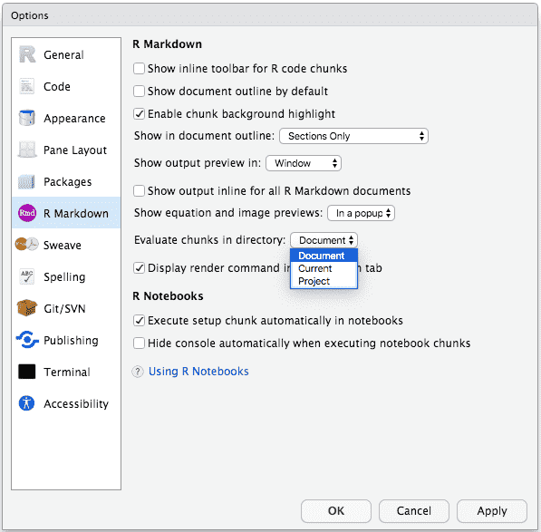
FIGURE 16.1: Change the default working directory for all R Markdown documents in RStudio.
In RStudio, you may also knit an individual Rmd document with a specific working directory, as shown in Figure 16.2. After you change the “Knit Directory” and click the “Knit” button, knitr will use the new working directory to evaluate your code chunks. All these settings boil down to knitr::opts_knit$set(root.dir = ...) as we mentioned earlier, so if you are not satisfied by any of these choices, you can specify a directory by yourself with knitr::opts_knit$set().
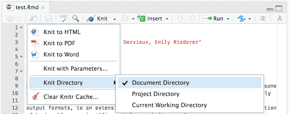
FIGURE 16.2: Knit an Rmd document with other possible working directories in RStudio.
There is no absolutely correct choice for the working directory. Each choice has its own pros and cons:
If you use the Rmd document directory as the working directory for code chunks (knitr’s default), you assume that file paths are relative to the Rmd document. This is similar to how web browsers handle relative paths, e.g., for an image
<img src="foo/bar.png" />on an HTML pagehttps://www.example.org/path/to/page.html, your web browser will try to fetch the image fromhttps://www.example.org/path/to/foo/bar.png. In other words, the relative pathfoo/bar.pngis relative to the directory of the HTML file, which ishttps://www.example.org/path/to/.The advantage of this approach is that you can freely move the Rmd file together with its referenced files anywhere, as long as their relative locations remain the same. For the HTML page and image example above, the files
page.htmlandfoo/bar.pngcould be moved together to a different directory, such ashttps://www.example.org/another/path/, and you will not need to update the relative path in thesrcattribute of<img />.Some users like to think of relative paths in Rmd documents as “relative to the working directory of the R console,” as opposed to “relative to the Rmd file.” Therefore knitr’s default working directory feels confusing. The reason that I did not use the working directory of the R console as the default when I designed knitr was that users could use
setwd()to change the working directory at any time. This working directory is not guaranteed to be stable. Each time a user callssetwd()in the console, there is a risk that the file paths in the Rmd document may become invalid. It could be surprising that the file paths depend on an external factor (setwd()), which is out of the control of the Rmd file. If you treat the Rmd file as “the center of the universe” when thinking of relative paths, the paths inside the Rmd file may be stabler.Furthermore, if you do not want to think too hard on relative paths, you may enter a path in RStudio using its autocomplete, as shown in Figure 16.3. RStudio will try to autocomplete a path relative to the Rmd file.
Using the working directory of the R console can be a good choice for knitting documents programmatically or interactively. For example, you may knit a document multiple times in a loop, and use a different working directory each time to read a different data file (with the same filename) in that directory. This type of working directory is advocated by the ezknitr package (Attali 2023), which essentially uses
knitr::opts_knit$set(root.dir)to change the working directory for code chunks in knitr.Using the project directory as the working directory requires an obvious assumption: you have to use a project (e.g., an RStudio project or a version control project) in the first place, which could be a disadvantage of this approach. The advantage of this type of working directory is that all relative paths in any Rmd document are relative to the project root directory, so you do not need to think where your Rmd file is located in the project or adjust the relative paths of other files accordingly. This type of working directory is advocated by the here package (Müller 2025), which provides the function
here::here()to return an absolute path by resolving a relative path passed to it (remember that the relative path is relative to the project root). The disadvantage is that when you move the referenced file together with the Rmd file to another location in the project, you need to update the referenced path in the Rmd document. When you share the Rmd file with other people, you also have to share the whole project.These types of paths are similar to absolute paths without the protocol or domain in HTML. For example, an image
<img src="/foo/bar.png" />on the pagehttps://www.example.org/path/to/page.htmlrefers to the image under the root directory of the website, i.e.,https://www.example.org/foo/bar.png. The leading/in thesrcattribute of the image indicates the root directory of the website. If you want to learn more (or further confuse yourself) about absolute and relative paths in HTML, please see Appendix B.1 of the blogdown book (Xie, Hill, and Thomas 2017).
The working directory pain mainly arises from this question when dealing with relative paths: relative to what? As we mentioned earlier, different people have different preferences, and there is not an absolutely right answer.
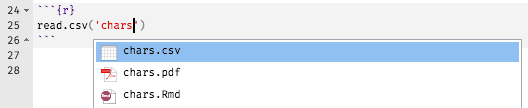
FIGURE 16.3: Autocomplete file paths in an Rmd document in RStudio.