2.2 R Markdown anatomy
We can dig one level deeper by considering the different components of an R Markdown. Specifically, let’s look at when and how these are altered during the rendering workflow.
2.2.1 YAML metadata
The YAML metadata (also called the YAML header) is processed in many stages of the rendering process and can influence the final document in many different ways. It is placed at the very beginning of the document and is read by each of Pandoc, rmarkdown, and knitr. Along the way, the information that it contains can affect the code, content, and the rendering process.
A typical YAML header looks like this, and contains basic metadata about the document and rendering instructions:
---
title: My R Markdown Report
author: Yihui Xie
output: html_document
---
In this case, the title and author fields are processed by Pandoc to set the values of template variables. With the default template, the title and author information will appear at the beginning of the resulting document. More details on how Pandoc uses information from the YAML header are included in the Pandoc manual’s section on the YAML metadata block.
In contrast, the output field is used by rmarkdown to apply the output format function rmarkdown::html_document() in the rendering process. We can further influence the rendering process by passing arguments to the output format that we are specifying in output. For example, writing:
output:
  html_document:
    toc: true
    toc_float: true
is the equivalent of telling rmarkdown::render() to apply the output format rmarkdown::html_document(toc = TRUE, toc_float = TRUE). To find out what these options do, and to learn about other possible options, you may run ?rmarkdown::html_document in your R console and read the help page. Note that output: html_document is equivalent to output: rmarkdown::html_document. When an output format does not have a qualifier like rmarkdown::, it is assumed that it is from the rmarkdown package, otherwise it must be prefixed with the R package name, e.g., bookdown::html_document2.
The YAML header can also influence our content and code if we choose to use parameters in YAML, as described in Section 17.4. In short, we can include variables and R expressions in this header that can be referenced throughout our R Markdown document. For example, the following header defines start_date and end_date parameters, which will be reflected in a list called params later in the R Markdown document. Thus, if we want to use these values in our R code, we can access them via params$start_date and params$end_date.
---
title: My RMarkdown
author: Yihui Xie
output: html_document
params:
  start_date: '2020-01-01'
  end_date: '2020-06-01'
---
2.2.2 Narrative
The narrative textual elements of R Markdown may be simpler to understand than the YAML metadata and code chunks. Typically, this will feel quite a bit like writing in a text editor. However, this Markdown content can be more powerful and interesting than simple text—both in how its content is made, and how the document structure is made from it.
While much of our narrative is human-written, many R Markdown documents will likely wish to reference the code and analysis being used. For this reason, Chapter 4 demonstrates the many ways that code can help generate parts of the text, such as combining words into a list (Section 4.11) or writing a bibliography (Section 4.5). This conversion is handled by knitr as we convert from .Rmd to .md.
Our Markdown text can also provide structure to the document. While we do not have enough space here to review the Markdown syntax,3 one particularly relevant concept is section headers, which are denoted by one or more hashes (#) corresponding to different levels, e.g.,
# First-level header

## Second-level header

### Third-level header
These headers give structure to our entire document as rmarkdown converts the .md to our final output format. This structure is useful for referencing and formatting these sections by appending certain attributes to them. To create such references, Pandoc syntax allows us to provide a unique identifier by following the header notation with {#id}, or attach one or more classes to a section with {.class-name}, e.g.,
## Second-level header {#introduction .important .large}We can then access this section with many of the tools that you will learn, e.g., by referencing it with its ID or class. As examples, Section 4.7 demonstrates how to use the section ID to make cross-references throughout your document, and Section 7.6 introduces the .tabset class to help reorganize subsections.
The final interesting type of content that we might find in the textual part of our R Markdown is raw content written specifically for our desired output format, e.g., raw LaTeX code for LaTeX output (Section 6.11), raw HTML code for HTML output, and so on (Section 9.5). Raw content may help you achieve things that cannot be done with plain Markdown, but please keep in mind that it is usually ignored when the output format is a different format, e.g., raw LaTeX commands in Markdown will be ignored when the output format is HTML.
2.2.3 Code chunks
Code chunks are the beating heart of our R Markdown. The code in these chunks is run by knitr, and its output is translated to Markdown to dynamically keep our reports in sync with our current scripts and data. Each code chunk consists of a language engine (Chapter 15), an optional label, chunk options (Chapter 11), and code.
To understand some of the modifications that we can make to code chunks, it is worth understanding the knitr process in slightly more detail. For each chunk, a knitr language engine gets three pieces of input: the knitting environment (knitr::knit_global()), the code input, and a list of chunk options. It returns the formatted representations of the code as well as its output. As a side effect, the knitting environment may also be modified, e.g., new variables may have been created in this environment via the source code in the code chunk. This process is illustrated in Figure 2.2.
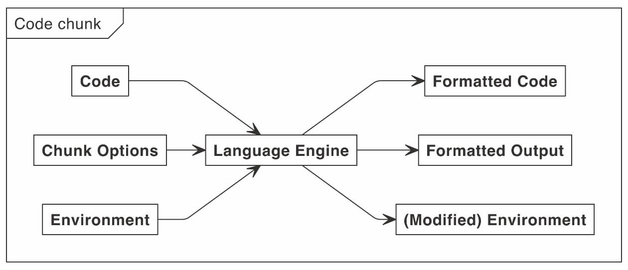
FIGURE 2.2: A flowchart of inputs and outputs to a language engine.
We can modify this process by:
changing our language engine;
modifying chunk options, which can be global, local, or engine-specific;
and by using hooks (Chapter 12 and Chapter 13) to further process these inputs and outputs.
For example, in Section 12.1, you will learn how to add a hook to post-process the code output to redact certain lines in the source code.
Code chunks also have analogous concepts to the classes and unique identifiers that we explored for narratives in Section 2.2.2. A code chunk can specify an optional identifier (often called the “chunk label”) immediately after its language engine. It can set classes for code and text output blocks in the output document via the chunk options class.source and class.output, respectively (see Section 7.3). For example, the chunk header ```{r summary-stats, class.output = 'large-text'} gives this chunk a label summary-stats, and the class large-text for the text output blocks. A chunk can have only one label, but can have multiple classes.
2.2.4 Document body
One important thing to understand when authoring and modifying a document is how code and narrative pieces create different sections, or containers within the document. For example, suppose we have a document that looks like this:
# Title

## Section X

This is my introduction.

```{r chunk-x}
x <- 1
print(x)
```

### Subsection 1

Here are some details.

### Subsection 2

These are more details.

## Section Y

This is another section.

```{r chunk-y}
y <- 2
print(y)
```
When writing this document, we might think of each piece as linear with independent sections of text and code following in a sequence one after the other. However, what we are actually doing is creating a set of nested containers that conceptually4 looks more like Figure 2.3.
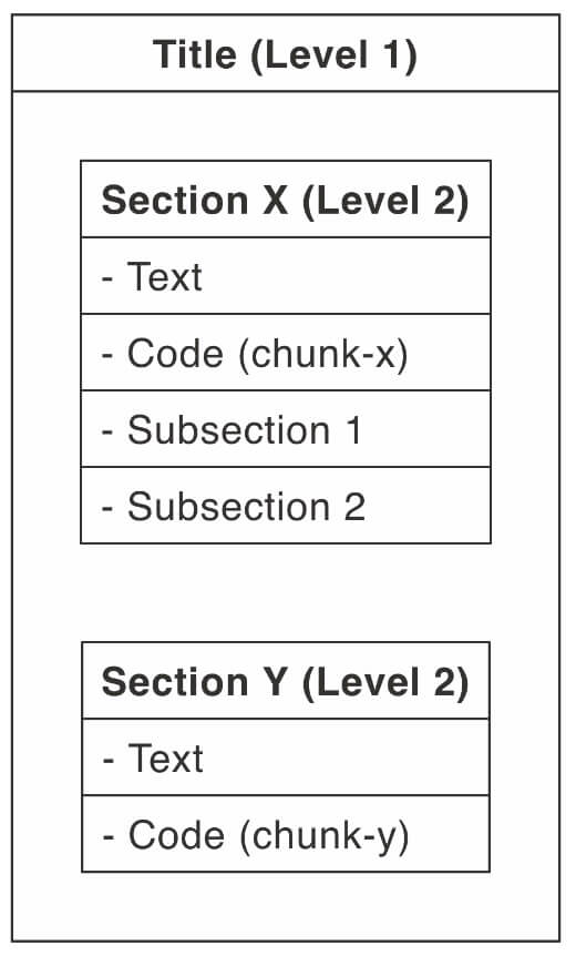
FIGURE 2.3: A simple R Markdown document illustrated as a set of nested containers.
Two key features of this diagram are (1) every section of text or code is its own discrete container, and (2) containers can be nested within one another. This nesting is particularly apparent if you are authoring your R Markdown document in the RStudio IDE and expand the document outline.
Note that in Figure 2.3, headers of the same level represent containers at the same level of nesting. Lower-level headers exist inside of the container of higher-level headers. In this case, it is common to call the higher-level sections the “parent” and the minor sections the “child.” For example, a subsection is the child of a section. Besides headers, you can also create divisions in your text using :::, as demonstrated in Section 5.8.
This structure has important implications as we attempt to apply some of the formatting and styling options that are described in this text. For example, we will see this nested structure when we learn about how Pandoc represents our document as an abstract syntax tree (Section 4.20), or when we use CSS selectors (Section 7.1, among others) to style our HTML output.
Formatting and styling can be applied to either containers of similar types (e.g., all code blocks), or all containers that exist inside of another container (e.g., everything under “Section Y”). Additionally, as explained in Section 2.2.2, we can apply the same classes to certain sections to designate them as being similar, and in this case, the common class names denote the common properties or intent of these sections.
As you read through this cookbook, it may be useful to quiz yourself and think about what sort of container the specific “recipe” is acting upon.
Instead, for a review of the Markdown syntax, please see https://bookdown.org/yihui/bookdown/markdown-syntax.html.↩︎
In reality, there are many more containers than shown. For example, for a knitted code chunk, the code and output exist in separate containers that share a common parent.↩︎